A Meshless Model of Rigid-Body Motion in Viscous Fluids

Modeling rigid particles in viscous flow gets difficult fast when body boundaries move and traditional meshes must follow. This article breaks down a meshless ISPH approach that keeps fluid and solid in one particle system, then enforces rigid motion through a projection step. I developed this analysis for my MATH*6051 poster presentation session. I focus on the Single Disc Descent benchmark, which is the calibration case that sets up the rest of the method.

The source study is An incompressible smoothed particle hydrodynamics method for the motion of rigid bodies in fluids by N. Tofighi, M. Ozbulut, A. Rahmat, J. J. Feng, and M. Yildiz, published in the Journal of Computational Physics, vol. 297, pp. 207-220 (2015). [1]

What problem this model solves

The paper models rigid particles moving through viscous Newtonian fluids. The target phenomena include settling under gravity, shear-induced rotation, lateral migration, and near-contact interaction between multiple bodies.

The core implementation goal is simple: keep the algorithm meshless and avoid explicit moving-body meshing.

The method does that by combining three ideas:

• Solve one incompressible SPH system on all particles.
• Represent the solid phase as a high-viscosity pseudo-fluid during the momentum solve.
• Project solid-particle velocities back to rigid-body motion after each step.

This lets the method stay in a single particle framework while still preserving rigid kinematics.

Assumptions and modeling scope

• 2D incompressible Newtonian flow.
• Diffuse fluid-solid transition produced by kernel smoothing.
• Cubic spline kernel for color smoothing.
• Quintic spline kernel for derivative operators.
• Rigid behavior enforced by a viscosity-penalty plus rigid-projection coupling.
• Validation range in the paper reaches about $Re_p=391$.

This is best suited for particulate-flow problems where moving-mesh approaches become expensive or fragile.

Key notation used throughout

To match the poster and paper notation, I use the same symbols and the same fluid/solid subscript convention.

Physical and rigid-body variables

Symbol	Meaning
$\rho,\mu,p,\mathbf{u},t$	density, dynamic viscosity, pressure, velocity, time
$\mathbf{r}_i,m_i$	particle position and mass
$\mathbf{u}_s^t,\mathbf{u}_s^r$	rigid-body translational and rotational velocities
$M_s,I_s$	rigid-body mass surrogate and inertia surrogate

Nondimensional groups and SPH fields

Symbol	Meaning
$\mathcal{D}=\rho_s/\rho_f$	density ratio
$\mathcal{V}=\mu_s/\mu_f$	viscosity ratio
$\mathrm{Re}=\rho_f u_c l_c/\mu_f$	Reynolds number
$d,h$	disc diameter and smoothing length
$W_{ij}=W(\mathbf{r}_{ij},h)$	interpolation kernel
$\mathbf{r}_{ij}=\mathbf{r}_i-\mathbf{r}_j$	particle separation vector
$\psi_i=\sum_j W_{ij}$	number density
$\hat{c}_i^\alpha,c_i^\alpha,c_i$	sharp and smoothed phase color functions
$\varphi_i$	blended material property ($\rho$ or $\mu$)

Discrete operators and algorithm symbols

Symbol	Meaning
$a_i^{ml}$	correction tensor in the discrete operators
$\phi_i,\phi_{ij}$	local transport property and harmonic pair mean
$f_i^m,f_i$	generic vector/scalar fields in operator formulas
$J_n,J_s,J_d$	neighbors, particles in one solid, particles in full domain
$\gamma$	CFL safety factor
$\delta\mathbf{r}_i$	artificial particle-shift displacement

Mathematical model in detail

1) Governing PDEs and scaling (Eqs. 1-5)

The paper solves dimensionless incompressible Navier-Stokes equations:

$$\nabla\cdot\mathbf{u}=0 \tag{1}$$

Equation (1) is the incompressibility constraint. It says the velocity field has no divergence anywhere, meaning no local compression or expansion. This will be enforced iteratively through the pressure solve rather than exactly at each step.

$$\rho\frac{D\mathbf{u}}{Dt}=-\nabla p + \frac{1}{\mathrm{Re}}\nabla\cdot\boldsymbol{\tau} \tag{2}$$ $$\boldsymbol{\tau}=\mu\left[\nabla\mathbf{u}+(\nabla\mathbf{u})^{\dagger}\right] \tag{3}$$

Equations (2) and (3) are the momentum equation and the Newtonian stress tensor. The critical point is that these are applied to all particles, fluid and solid alike. The solid is not given special treatment in the momentum solve. It is simply assigned a much higher viscosity $\mu_s = \mathcal{V}\mu_f$, which suppresses internal deformation and makes it behave approximately like a rigid body. The rigidity constraint is enforced separately afterward.

$$\mathrm{Re}=\frac{\rho_f u_c l_c}{\mu_f} \tag{5}$$

The Reynolds number uses fluid reference values only. For the SDD benchmark, the characteristic length is the disc diameter $d$ and the characteristic velocity is $\sqrt{gd}$, so $\mathrm{Re}_p = \rho_f\sqrt{gd}\cdot d/\mu_f$. Everything else in the formulation is then dimensionless relative to these scales.

2) Phase interpolation and diffuse interface (Eqs. 6-8)

Each phase $\alpha$ is identified by a sharp indicator $\hat{c}_j^\alpha \in \{0,1\}$. That indicator is smoothed over neighbors with the SPH kernel to produce a continuous phase color:

$$c_i^\alpha=\frac{1}{\psi_i}\sum_{j=1}^{J_n}\hat{c}_j^\alpha W_{ij} \tag{6}$$

The result is a value between 0 and 1 that varies smoothly across the fluid-solid interface over a few particle spacings. It is used to blend material properties at each particle. Two blending rules are compared:

$$\varphi_i=\sum_\alpha \varphi_s^\alpha c_i^\alpha + \varphi_f c_i \qquad \text{(WAM)} \tag{7}$$ $$\frac{1}{\varphi_i}=\sum_\alpha\frac{c_i^\alpha}{\varphi_s^\alpha}+\frac{c_i}{\varphi_f} \qquad \text{(WHM)} \tag{8}$$

WAM is a linear average weighted by phase fraction. WHM is its harmonic counterpart. For large $\mathcal{V}$, the two behave very differently at the interface. WAM’s linear blend allows the solid viscosity to dilute into the fluid region, making interface particles effectively softer than they should be. WHM, by contrast, is dominated by the smaller of the two values at any given point, which keeps the fluid-side properties nearly unaffected and concentrates the viscosity transition inside the solid boundary. This is why WHM is necessary at high $\mathcal{V}$ and why the SDD benchmark is used to verify it.

3) Rigid-body projection constraints (Eqs. 9-12)

After the momentum solve, the solid particles have velocities that vary across the body because the SPH solve treats them like fluid. The projection step collapses that variation back down to exactly the two degrees of freedom a 2D rigid body can have: translation and rotation.

First, a momentum-weighted average extracts the body’s translational velocity:

$$\mathbf{u}_s^t=\frac{1}{M_s}\sum_{j=1}^{J_s}\frac{\mathbf{u}_j}{\psi_j} \tag{9}$$

Then the angular velocity is recovered by computing the net angular momentum about the center of mass and dividing by the moment of inertia:

$$\mathbf{u}_s^r=\frac{1}{I_s}\sum_{j=1}^{J_s}\frac{\mathbf{u}_j\times\mathbf{r}_{js}}{\psi_j} \tag{10}$$

Finally, every solid particle’s velocity is overwritten with the rigid-body field:

$$\mathbf{u}_i=\mathbf{u}_s^t+\mathbf{u}_s^r\times\mathbf{r}_{is} \tag{11}$$

The normalizing quantities $M_s$ and $I_s$ are not mass and moment of inertia in the usual sense. They are number-density-weighted sums over the solid particles:

$$M_s=\sum_{j=1}^{J_s}\frac{1}{\psi_j}, \qquad I_s=\sum_{j=1}^{J_s}\frac{r_{js}^2}{\psi_j} \tag{12}$$

This is the mechanism that prevents solid particles from drifting as fluid-like points, particularly in the interface region where the diffuse smoothing reduces the effective viscosity contrast and the viscosity penalty alone is no longer sufficient.

4) Corrected SPH operators (Eqs. 13-17)

Standard SPH gradient operators lose first-order consistency on irregular particle distributions, which is exactly what you get near a moving interface. The paper uses a correction tensor $a_i^{ml}$ to restore consistency. The corrected gradient is defined implicitly by:

$$\frac{\partial f_i^m}{\partial x_i^k}a_i^{kl} =\sum_j\frac{1}{\psi_j}(f_j^m-f_i^m)\frac{\partial W_{ij}}{\partial x_i^l} \tag{13}$$

The right-hand side is a standard SPH gradient sum. Multiplying through by $a_i^{-1}$ recovers the corrected gradient. This makes the operator first-order consistent: it reproduces linear fields exactly regardless of how the particles are arranged.

The variable-coefficient Laplacian used for the viscous stress divergence in Eq. (2) follows the same corrected form:

$$\frac{\partial}{\partial x_i^k}\left(\phi_i\frac{\partial f_i^m}{\partial x_i^k}\right)a_i^{ml} =8\sum_j\frac{\phi_{ij}}{\psi_j}(f_i^m-f_j^m)\frac{r_{ij}^m}{r_{ij}^2}\frac{\partial W_{ij}}{\partial x_i^l} \tag{14}$$

The scalar version, used in the pressure Poisson equation, absorbs the trace of the correction tensor directly into the prefactor:

$$\frac{\partial}{\partial x_i^k}\left(\phi_i\frac{\partial f_i}{\partial x_i^k}\right)\left[2+a_i^{kk}\right] =8\sum_j\frac{\phi_{ij}}{\psi_j}(f_i-f_j)\frac{r_{ij}^k}{r_{ij}^2}\frac{\partial W_{ij}}{\partial x_i^k} \tag{15}$$

Both operators use the harmonic pair mean for the transport coefficient $\phi$:

$$\phi_{ij}=\frac{2\phi_i\phi_j}{\phi_i+\phi_j} \tag{16}$$

This is the same harmonic averaging principle that WHM uses for property interpolation. At the diffuse interface, where one side has $\mu_s = 100\mu_f$ and the other has $\mu_f$, a simple arithmetic mean would blow up the effective coefficient. The harmonic mean keeps it bounded and physically sensible, because it is pulled strongly toward the smaller of the two values.

The correction tensor itself is computed from a neighbor sum:

$$a_i^{ml}=\sum_j\frac{r_{ij}^m}{\psi_j}\frac{\partial W_{ij}}{\partial x_i^l} \tag{17}$$

On a perfectly uniform Cartesian grid, $a_i^{ml}$ would be the identity and nothing would change. On the real irregular particle distribution around a moving boundary, it provides the correction that keeps the gradient operator honest.

5) Time integration and projection cycle (Eqs. 18-26)

The timestep is CFL-limited by two competing constraints:

$$\Delta t=\gamma\min_{1\leq i\leq J_d}\left(\frac{h}{u_i},\frac{1}{\mathrm{Re}}\frac{h^2\rho_i}{2\mu_i}\right), \qquad \gamma=0.25 \tag{18}$$

The first term is the advection limit: a particle should not travel more than one smoothing length per step. The second is the viscous diffusion limit: momentum should not diffuse more than $O(h^2)$ per step. At the beginning of SDD, when everything is at rest, the advection limit goes to infinity and the viscous term alone controls the timestep. High viscosity ratios, large $\mathcal{V}$, tighten this limit further because $\mu_i$ is large for solid particles. This is exactly why the CPU simulation was so slow: at startup, the timestep is governed by viscosity rather than by any interesting flow, and it stays small for a long time.

The whole step is a predictor-corrector cycle. The predictor advances positions and velocities using only the known forces from the current timestep, ignoring pressure. The corrector then solves for a pressure field that removes the divergence the predictor introduced, and uses it to fix the velocities. Positions get a final update from the corrected velocities. Throughout, a superscript $+$ denotes the predicted (intermediate) state and $^{(n+1)}$ denotes the fully corrected end-of-step state.

Position predictor (Eq. 19):

$$\mathbf{r}_i^+=\mathbf{r}_i^{(n)}+\mathbf{u}_i^{(n)}\Delta t+\delta\mathbf{r}_i^{(n)} \tag{19}$$

A forward Euler advance of particle position. The extra $\delta\mathbf{r}_i^{(n)}$ term is the artificial particle shift described in Eq. (20). This predicted position is intermediate: it is used during the pressure solve but replaced by the final trapezoidal update in Eq. (26).

Artificial particle shift (Eq. 20):

$$\delta\mathbf{r}_i^{(n)}= \zeta\left[ \max_{1\leq k\leq J_d}(u_k)\sum_{j=1}^{J_n} \left(\frac{\mathbf{r}_{ij}}{r_{ij}^3}r_{av,j}^2\right) \right]^{(n)}\Delta t, \qquad \zeta=0.06 \tag{20}$$

SPH kernel accuracy degrades when particles cluster unevenly. This term prevents that by nudging each particle away from its neighbors. The direction of the push is $\mathbf{r}_{ij}/r_{ij}^3$: a unit vector pointing from neighbor $j$ toward $i$, weighted by inverse-square distance so that close neighbors exert a stronger repulsion. The factor $r_{av,j}^2$ scales the shift by the square of the local mean inter-particle spacing, making it proportional to how crowded the neighborhood is rather than to any absolute distance. The whole expression is then scaled by the global maximum velocity $\max(u_k)$ and $\Delta t$, so the shift remains small relative to the flow even at coarse timesteps. The coefficient $\zeta = 0.06$ is empirically set to keep the shift from distorting the physics while still regularizing the particle distribution.

Velocity predictor (Eq. 21):

$$\mathbf{u}_i^+=\mathbf{u}_i^{(n)}+\frac{1}{\rho^{(n)}\mathrm{Re}}\nabla\cdot\boldsymbol{\tau}_i^{(n)}\Delta t \tag{21}$$

The velocity is advanced by the viscous stress divergence alone. Pressure is deliberately excluded here. This is the defining feature of the ISPH projection approach: the predictor handles all the physics that does not enforce incompressibility, leaving pressure as a corrector-step quantity. The viscous term $\nabla\cdot\boldsymbol{\tau}$ is computed using the corrected Laplacian from Eq. (14), with harmonic-mean pair coefficients to handle the sharp viscosity contrast at the fluid-solid interface.

Number density and density update (Eqs. 22-23):

$$\psi_i^+=\psi_i^{(n)}-\Delta t\,\psi_i^{(n)}(\nabla\cdot\mathbf{u}_i^+) \tag{22}$$ $$\rho_i^+=m_i\psi_i^+ \tag{23}$$

The predicted velocity field $\mathbf{u}^+$ is not yet divergence-free, so it would compress or expand the local particle distribution if left uncorrected. Eq. (22) tracks that effect by advancing the number density $\psi_i$ forward in time using $\nabla\cdot\mathbf{u}^+$ as a source. The updated density $\rho_i^+$ follows immediately from $\rho = m\psi$. These predicted densities appear in the coefficient $1/\rho^+$ of the pressure Poisson equation and in the velocity correction, ensuring the projection step is consistent with the density state the particles would actually reach.

Pressure projection:

$$\nabla\cdot\left(\frac{1}{\rho^+}\nabla p^{(n+1)}\right)=\frac{\nabla\cdot\mathbf{u}^+}{\Delta t} \tag{24}$$

The right-hand side is the divergence of the predicted velocity, which measures exactly how much $\mathbf{u}^+$ violates incompressibility. The pressure field $p^{(n+1)}$ is solved so that subtracting its gradient from $\mathbf{u}^+$ drives that divergence to zero. The variable-coefficient operator on the left uses the predicted density $\rho^+$, making the effective pressure stiffness spatially non-uniform across the diffuse fluid-solid interface. The equation is solved iteratively via Jacobi iteration using the discrete Laplacian from Eq. (15).

Velocity correction (Eq. 25):

$$\mathbf{u}^{(n+1)}=\mathbf{u}^+-\frac{1}{\rho^+}\nabla p^{(n+1)}\Delta t \tag{25}$$

The pressure gradient is subtracted from the predicted velocity, projecting it onto the space of divergence-free fields. This is the corrector step. After this, $\mathbf{u}^{(n+1)}$ satisfies $\nabla\cdot\mathbf{u}\approx 0$ to the tolerance of the iterative solver.

Final position update (Eq. 26):

$$\mathbf{r}_i^{(n+1)}=\mathbf{r}_i^{(n)}+\frac{1}{2}\left(\mathbf{u}_i^{(n)}+\mathbf{u}_i^{(n+1)}\right)\Delta t+\delta\mathbf{r}_i^{(n)} \tag{26}$$

Rather than using the predicted velocity from Eq. (19), the final position is computed with a trapezoidal average of the old and new velocities. This gives second-order temporal accuracy in position even though the velocity advance itself is first-order. The artificial shift $\delta\mathbf{r}_i^{(n)}$ is applied here consistently with the predictor position in Eq. (19).

After Eq. (25), the rigid-body projection (Eqs. 9-11) is applied to solid particles before the position update. This overwrites the corrected velocities for the solid with a strictly rigid field, which technically re-introduces a small divergence near the interface. The authors acknowledge this explicitly: the incompressibility condition is temporarily violated at the fluid-solid boundary and corrected in the next pressure solve. It is a deliberate design choice that keeps the algorithm simple. One momentum solve, one projection; at the cost of a small per-step interface error that is then cleaned up.

Single Disc Descent (SDD): full benchmark analysis

Why SDD is the key calibration case

SDD is not only a validation example. It is the case used to choose interpolation strategy and viscosity ratio for the entire study.

The question is: as $\mathcal{V}=\mu_s/\mu_f$ increases, does the solid approach rigid settling behavior in a stable, convergent way?

Case definition in the paper

• Disc released from rest in a quiescent fluid.
• Characteristic scales: $l_c=d$, $u_c=\sqrt{gd}$.
• Governing dimensionless groups: $Re_p$, $h/d$, $\mathcal{D}$, and $\mathcal{V}$.
• Calibration settings for Table 1: $Re_p=39.1$, $h/d=16$, $\mathcal{D}=1.25$, sampled at $t=30$.

Domain and discretization details reported by the authors:

• Rectangular domain with no-slip and no-penetration walls.
• Solid represented by concentric circular particle layers.
• Fluid initialized on a Cartesian particle grid.
• Initial local nonuniformity near the disc is corrected by the shifting and projection steps.

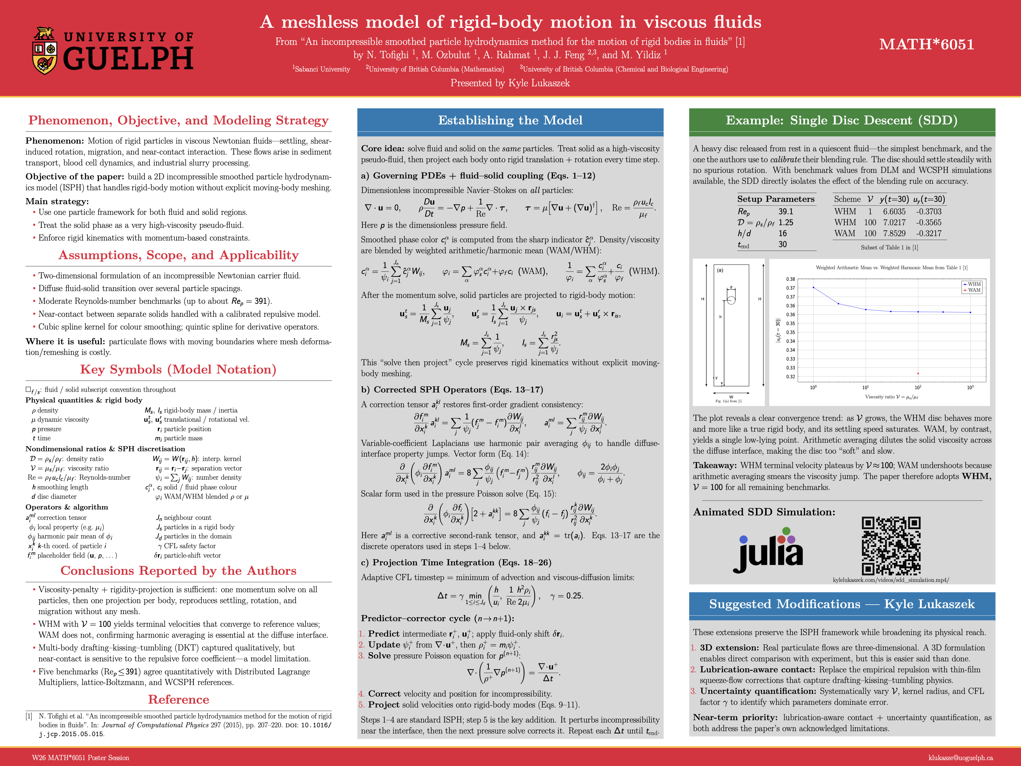
Table 1 values (paper data)

Scheme	$\mathcal{V}$	$y(t=30)$	$u_y(t=30)$
WHM	1	6.6035	-0.3703
WHM	3	6.8568	-0.3611
WHM	10	6.9818	-0.3578
WHM	30	7.0091	-0.3567
WHM	100	7.0217	-0.3565
WHM	300	7.0279	-0.3564
WHM	1000	7.0262	-0.3562
WAM	100	7.8529	-0.3217

What the numbers show

For WHM, $u_y(t=30)$ approaches a plateau as $\mathcal{V}$ grows. The change from $\mathcal{V}=30$ to $\mathcal{V}=1000$ is tiny relative to the change from $\mathcal{V}=1$ to $\mathcal{V}=30$. That is the convergence behavior expected when the solid limit is being approached.

WAM at $\mathcal{V}=100$ produces a much smaller velocity magnitude than WHM at the same ratio, indicating the effective solid response is too soft at the interface. The authors attribute this to arithmetic blending smearing the viscosity jump.

This is why the paper adopts WHM with $\mathcal{V}=100$ for the remaining cases.

Resolution and timestep checks reported in SDD

The paper studies multiple spatial resolutions in SDD and reports:

• Convergence in vertical velocity between higher resolutions.
• Position differences that remain controlled across refined runs.
• A practical resolution choice of $J_d=62{,}230$.

For the CFL factor $\gamma$:

• $\gamma=0.125$ and $\gamma=0.25$ agree closely.
• $\gamma=0.5$ gives noticeably slower descent.

Thus the baseline setting used through the study is $\gamma=0.25$.

Comparison with prior reference methods

Using the calibrated setup, the SDD trajectories are compared against WCSPH (Hashemi et al.) and DLM (Glowinski et al.).

Reported behavior:

• Overall quantitative agreement across acceleration, near-terminal descent, and wall-influenced deceleration stages.
• Small differences in when boundary effects appear and in fine details of transients.
• Terminal settling behavior remains in strong agreement, especially with DLM trends.

SDD simulation video

Simulating in Julia

I first implemented this in Float64: a paper-faithful, multithreaded Julia solver where each equation from the source has a corresponding function, and each particle is a mutable struct with its own heap-allocated position and velocity vectors.

mutable struct Particle
    id::Int
    x::Vector{Float64}
    u::Vector{Float64}
    u_plus::Vector{Float64}
    p::Float64
    rho::Float64
    mu::Float64
    psi::Float64
    is_solid::Bool
    delta_r::Vector{Float64}
    # ...
end

It was seemingly correct across the frames that I tested, and it ran at about 300 ms per timestep on a multithreaded CPU.

That sounds fine until you do the math. SDD uses an adaptive CFL timestep: the solver picks $\Delta t$ based on the fastest particle in the domain at each step. At the start of SDD, the disc is at rest and nothing is moving. The timestep is determined almost entirely by the viscous diffusion limit rather than advection, which keeps it very small. Over a full run to $t=50$, that adds up to millions of steps just to watch a disc fall.

At 300 ms a step, one second of 20 fps animation required roughly 8 hours of wall-clock compute. In that first second of footage, almost nothing happens. The disc has barely begun to accelerate. Scientifically boring footage produced at a genuinely painful rate.

That’s when I rewrote it for the GPU using the Metal.jl Julia Package.

Array of Structs to Struct of Arrays

Metal kernels are data-parallel: thousands of threads run the same function simultaneously, each reading from a shared array at their own index. The enemy of GPU throughput is scattered memory access. With the CPU Particle struct above, adjacent threads reading u[i] and u[i+1] are reading bytes that are a full struct-width apart in memory. Cache lines get wasted.

The fix is to split every field into its own flat array:

x::MtlVector{Float32}
y::MtlVector{Float32}
u::MtlVector{Float32}
v::MtlVector{Float32}
rho::MtlVector{Float32}
mu::MtlVector{Float32}
psi::MtlVector{Float32}
# ...

When a kernel reads x[i], threads i, i+1, i+2… are reading consecutive bytes from the same array. The GPU can serve 32 threads from a single cache line fetch instead of 32 separate requests.

CSR neighbor lists

The CPU neighbor lists are Vector{Vector{Int}}: each inner vector is a separately-allocated heap object. Following a neighbor reference requires two pointer dereferences. On GPU this is a memory access pattern disaster.

The Metal version uses Compressed Sparse Row (CSR) format: two flat arrays, nbr_ptr and nbr_idx.

k0 = Int(ptr[i])
k1 = Int(ptr[i + 1]) - 1
for k in k0:k1
    j = Int(idx[k])
    # use neighbor j
end

This is one contiguous allocation. Iterating over neighbors of particle $i$ is a sequential read starting at nbr_ptr[i], which is exactly what a GPU cache wants.

The kernel gradients $\nabla W_{ij}$ and the Laplacian coefficient $({\mathbf{r}_{ij} \cdot \nabla W_{ij}}) / {|\mathbf{r}_{ij}|^2}$ are precomputed during the neighbor build and stored in matching CSR arrays gwx, gwy, qcoef. GPU kernels that need them just index into a flat array.

What got dropped

A few things were deliberately cut to keep the GPU kernels simple.

The corrective tensor $a_i^{ml}$ (Eq. 17) restores first-order gradient consistency near irregular particle distributions and appears in the gradient and Laplacian operators throughout the CPU version. In the Metal version it is gone. The Laplacian in the predictor kernel is the raw harmonic-mean form:

muij = (2f0 * mui * muj) / max(mui + muj, EPS_DIV)
coeff = 8f0 * muij * ipsi[j] * qcoef[k]
lap_u += (ui - u[j]) * coeff
lap_v += (vi - v[j]) * coeff

One tight loop, no matrix solve. ipsi[j] is the precomputed reciprocal number density $1/\psi_j$, computed once per step by a dedicated kernel_compute_ipsi! dispatch and reused across all kernels. The harmonic mean viscosity is the important part for the diffuse-interface physics; the correction tensor buys accuracy near irregular distributions, but it costs another full neighbor pass and a 2×2 system per particle.

The pressure Jacobi runs a fixed iteration count instead of checking residuals. A convergence check requires a global max-reduction across all 62,000 particles, then a synchronization, then a branch. At this problem size, the overhead rivals the cost of just running a few extra sweeps. The fixed count also means the step function is fully predictable in terms of GPU dispatch count, which helps throughput.

Rather than submitting one command buffer per Jacobi iteration, the solver uses a fused kernel that loops internally. kernel_pressure_jacobi_fused! accepts a half_iters parameter and ping-pongs between two pressure buffers inside a single dispatch, eliminating the per-iteration CPU round-trip entirely. The result always lands back in the primary buffer, so no pointer swap is needed afterward.

The CPU version initializes a full layer of ghost particles with negative IDs that ghost the domain walls and participate in all neighbor queries. The Metal version drops all of that and just clamps positions and damps velocities near walls on the CPU advection pass. No extra particles, no extra neighbor query cost, and nothing the animation makes visible.

What stays on CPU

Not everything belongs on the GPU.

The neighbor build uses a spatial hash grid and dictionary insertion that is inherently sequential. GPU atomics would slow it down at this scale. The CPU builds the CSR arrays and uploads them to the GPU. A skin-distance check amortizes the rebuild cost: the neighbor list is only regenerated when any particle has moved more than half the skin radius from its reference position at the last rebuild, or after a fixed maximum number of steps. Steps that reuse an existing list skip the build entirely.

The rigid-body projection (Eqs. 9-11) is a global reduction over solid particles: sum momenta, find center of mass, compute angular velocity, write back corrected velocities. There are only a few hundred solid particles in SDD. Dispatching a GPU reduction for a few hundred elements would spend more time in overhead than in math.

# Stays on CPU, runs over ~hundreds of solid particles
utx_num += state.u_h[i] * invpsi
uty_num += state.v_h[i] * invpsi
omega_num += (state.u_h[i] * ry - state.v_h[i] * rx) * invpsi

So each step conditionally rebuilds and uploads neighbor data, uploads particle state to the GPU, runs seven kernels, synchronizes, then pulls velocities back to the CPU for the rigid-body projection before writing positions.

The step loop

That sequence is visible directly in the step! function:

function step!(state::SimulationState)
    dt, _, _ = estimate_dt(state)

    if should_rebuild_neighbors(state)
        build_neighbor_csr!(state, 3f0 * h(p) + skin)  # CPU, uploads CSR to GPU
    end
    update_device_state!(state)  # x, y, u, v → GPU

    threads = 256
    groups  = cld(state.n, threads)

    @metal threads=threads groups=groups kernel_properties!(...)      # psi, rho, mu, c_solid
    @metal threads=threads groups=groups kernel_compute_ipsi!(...)    # ipsi = 1/psi
    @metal threads=threads groups=groups kernel_predictor!(...)       # u+, v+  (viscous advance)
    @metal threads=threads groups=groups kernel_divergence!(...)      # ∇·u+, rhs

    fill!(state.p, 0f0); fill!(state.p_new, 0f0)
    @metal threads=threads groups=groups kernel_pressure_jacobi_fused!(...)  # loops half_iters internally

    @metal threads=threads groups=groups kernel_correct_velocity!(...)  # u, v ← u+ - dt∇p/ρ
    synchronize()

    update_host_velocity_psi!(state)   # u, v, psi ← GPU
    impose_rigidity!(state)            # CPU: Eqs. 9-11, solid projection (~280 particles)

    @metal threads=threads groups=groups kernel_artificial_shift!(...)  # δr → GPU
    synchronize()
    copyto!(state.shift_x_h, state.shift_x)
    copyto!(state.shift_y_h, state.shift_y)

    advect_and_apply_walls!(state, dt) # CPU: positions + clamp-and-damp walls
end

Seven @metal dispatches, 62,000 threads each. The pressure kernel is the most expensive: it loops half_iters times internally over the full neighbor list, with no command-buffer round-trip between iterations. The artificial particle shift, previously a CPU neighbor walk over all fluid particles, now runs as a GPU kernel after the rigid-body projection — the projection result feeds umax as a scalar to the kernel, so no additional download is required. After the final synchronize(), the only CPU work is advection and wall enforcement.

Float32 was not optional

Metal shaders run in Float32. There is no Float64 on Apple Silicon Metal: not available, not a toggle. The precision reduction was not a design choice; it came with the GPU.

The practical consequence is faster accumulation of pressure and interface error over long runs. The solver needs explicit $\Delta t$ clamps and optional stability guards that the Float64 version never required. Float64 at $10^{-15}$ precision is forgiving. Float32 at $10^{-7}$ is not.

Results

The quantitative results do not match the paper’s Table 1 curves exactly. Dropped corrective tensors, fixed Jacobi iterations, simplified boundary treatment, and Float32 arithmetic all push the disc trajectory away from the reference. The visual behavior is correct: the disc falls, the wake develops, the settling is stable.

Getting to that footage without the GPU rewrite would have taken the better part of a month.

Why the paper still includes four more benchmarks

This post focuses numerically on SDD. The remaining cases exist to test distinct failure modes that SDD alone cannot cover:

• DDD (Double Disc Descent): checks multi-body interaction and near-contact behavior, especially Drafting-Kissing-Tumbling sensitivity to contact modeling.
• SDR (Single Disc Rotation): isolates rotational accuracy in shear flow and verifies $\omega/G$ behavior over Reynolds number.
• SDM (Single Disc Migration): verifies coupled translation and rotation in shear without body force.
• SED (Single Ellipse Descent): verifies non-circular rigid geometry, orientation dynamics, and terminal-state behavior.

Author conclusions

The paper validates the method across five benchmarks at $Re_p \leq 391$ and arrives at four main conclusions.

The viscosity-penalty plus rigidity-projection coupling is sufficient. One momentum solve over all particles followed by one rigid projection per body reproduces settling, shear-induced rotation, and lateral migration without any mesh. The diffuse interface does not need to be exact; the projection step absorbs the residual error.

WHM converges to the rigid limit; WAM does not. At $\mathcal{V}=100$, the WHM terminal velocities in Table 1 are nearly indistinguishable from $\mathcal{V}=300$ and $\mathcal{V}=1000$. WAM at the same ratio produces a meaningfully different trajectory, and not a better one. This is the central numerical result of SDD: harmonic averaging is not a cosmetic choice at the diffuse interface; arithmetic averaging underestimates the effective viscosity contrast and produces a body that is too compliant.

Multi-body behavior is captured qualitatively. The Double Disc Descent case reproduces the Drafting-Kissing-Tumbling sequence seen in experiment and in reference simulations. Near-contact behavior is sensitive to the repulsive force coefficient, which is an acknowledged model limitation. The method does not include lubrication physics, so very close particle approach relies entirely on a tuned empirical term.

Quantitative agreement with reference solvers. Across SDD, DDD, SDR, SDM, and SED, the ISPH results agree with Distributed Lagrange Multiplier (DLM), lattice-Boltzmann, and WCSPH references. Terminal velocities, rotation rates, and trajectory shapes fall within the spread of prior methods. The authors treat this as confirmation that the viscosity-penalty approach is a viable alternative to immersed-boundary and fictitious-domain formulations for particulate flow at moderate Reynolds numbers.

Suggested model extensions

Based on the paper limitations and my poster discussion:

• Extend to 3D particulate configurations.
• Replace empirical near-contact repulsion with lubrication-aware contact physics.
• Run structured uncertainty quantification over $\mathcal{V}$, kernel support, and $\gamma$.

Poster

Reference

[1] Tofighi, N., Ozbulut, M., Rahmat, A., Feng, J. J., & Yildiz, M. (2015). An incompressible smoothed particle hydrodynamics method for the motion of rigid bodies in fluids. Journal of Computational Physics, 297, 207-220. https://doi.org/10.1016/j.jcp.2015.05.015