Exploring Reinforcement Learning and Classification Algorithms
This article explores Q-learning for grid world navigation, Naive Bayes classification for text categorization, and Gaussian Mixture Models for clustering.
Setup
import gym
import numpy as np
import pandas as pd
import matplotlib.pyplot as plt
from mpl_toolkits.mplot3d import Axes3D
from sklearn.metrics import f1_score, accuracy_score, silhouette_score
from sklearn.mixture import GaussianMixture
Part 1: Grid World with Q-Learning
Grid World Environment
A 10x10 grid with open spaces (‘O’), obstacles (‘X’), a start (‘S’), and a goal (‘G’).
grid = [
    ['O', 'O', 'X', 'O', 'O', 'O', 'O', 'X', 'O', 'G'],
    ['O', 'X', 'X', 'X', 'O', 'X', 'O', 'X', 'O', 'O'],
    ['O', 'O', 'O', 'O', 'O', 'X', 'O', 'X', 'O', 'X'],
    ['O', 'X', 'X', 'X', 'O', 'X', 'O', 'X', 'O', 'O'],
    ['O', 'O', 'X', 'O', 'O', 'X', 'O', 'X', 'X', 'O'],
    ['O', 'O', 'X', 'X', 'O', 'X', 'O', 'O', 'O', 'O'],
    ['O', 'X', 'O', 'X', 'O', 'O', 'O', 'X', 'X', 'O'],
    ['O', 'X', 'O', 'X', 'O', 'X', 'O', 'X', 'O', 'O'],
    ['O', 'X', 'O', 'O', 'O', 'X', 'O', 'X', 'O', 'O'],
    ['O', 'O', 'O', 'X', 'O', 'O', 'S', 'O', 'O', 'O']
]

class GridWorld(gym.Env):
    def __init__(self, grid_layout):
        self.grid_layout = grid_layout
        self.rows = len(grid_layout)
        self.cols = len(grid_layout[0])
        self.goal_pos = self._find_pos('G')
        self.agent_pos = self._find_pos('S')
        self.agent_path = [self.agent_pos]
        self.steps = 0

        self.actions_map = {0: 'UP', 1: 'DOWN', 2: 'LEFT', 3: 'RIGHT'}
        self.action_space = gym.spaces.Discrete(4)
        self.observation_space = gym.spaces.Tuple((
            gym.spaces.Discrete(self.rows),
            gym.spaces.Discrete(self.cols)
        ))

        self.open_space_reward = -1
        self.obstacle_reward = -10
        self.goal_reward = 10

    def _find_pos(self, char):
        for i in range(self.rows):
            for j in range(self.cols):
                if self.grid_layout[i][j] == char:
                    return (i, j)
        return None

    def _is_valid_pos(self, i, j):
        return (0 <= i < self.rows and
                0 <= j < self.cols and
                self.grid_layout[i][j] != 'X')

    def _get_reward(self, i, j):
        if not self._is_valid_pos(i, j):
            return self.obstacle_reward
        elif (i, j) == self.goal_pos:
            return self.goal_reward
        else:
            return self.open_space_reward

    def _move_agent(self, action_idx):
        action = self.actions_map[action_idx]
        next_i, next_j = self.agent_pos

        if action == 'UP': next_i -= 1
        elif action == 'DOWN': next_i += 1
        elif action == 'LEFT': next_j -= 1
        elif action == 'RIGHT': next_j += 1

        reward = self._get_reward(next_i, next_j)

        if self._is_valid_pos(next_i, next_j):
            self.agent_pos = (next_i, next_j)
            self.agent_path.append(self.agent_pos)

        return reward

    def step(self, action_idx):
        reward = self._move_agent(action_idx)
        self.steps += 1
        done = (self.agent_pos == self.goal_pos)
        return self.agent_pos, reward, done, {}

    def reset(self):
        self.agent_pos = self._find_pos('S')
        self.agent_path = [self.agent_pos]
        self.steps = 0
        return self.agent_pos, {}

    def render(self, mode='human'):
        plt.figure(figsize=(self.cols, self.rows))

        traversed_grid = np.zeros((self.rows, self.cols))
        for r, c in self.agent_path:
            traversed_grid[r, c] = 1

        plt.imshow(traversed_grid, cmap='Blues', origin='upper', alpha=0.3)

        for r in range(self.rows):
            for c in range(self.cols):
                char = self.grid_layout[r][c]
                color = 'black'
                if char == 'X': color = 'red'
                elif char == 'S': color = 'green'
                elif char == 'G': color = 'orange'
                plt.text(c, r, char, ha='center', va='center', color=color, fontweight='bold')

        if len(self.agent_path) > 1:
            path_y, path_x = zip(*self.agent_path)
            plt.plot(path_x, path_y, color='black', linewidth=2, marker='o', markersize=3)

        plt.xticks([])
        plt.yticks([])
        plt.title(f"Agent Path - Steps: {self.steps}")
        plt.show()
Q-Learning Agent
class QLearningAgent:
    def __init__(self, num_actions, epsilon, gamma, alpha):
        self.num_actions = num_actions
        self.epsilon = epsilon
        self.alpha = alpha
        self.gamma = gamma
        self.q_table = {}

    def get_q_value(self, state, action_idx):
        if state not in self.q_table:
            self.q_table[state] = np.zeros(self.num_actions)
        return self.q_table[state][action_idx]

    def update_q_value(self, state, action_idx, reward, next_state):
        current_q = self.get_q_value(state, action_idx)

        if next_state not in self.q_table:
            self.q_table[next_state] = np.zeros(self.num_actions)

        max_next_q = np.max(self.q_table[next_state])
        new_q = current_q + self.alpha * (reward + self.gamma * max_next_q - current_q)
        self.q_table[state][action_idx] = new_q

    def choose_action(self, state):
        if np.random.rand() < self.epsilon:
            return np.random.choice(self.num_actions)
        else:
            if state not in self.q_table:
                self.q_table[state] = np.zeros(self.num_actions)
            return np.argmax(self.q_table[state])

def evaluate_q_learning(grid_layout, episodes, epsilon, gamma, alpha):
    env = GridWorld(grid_layout)
    agent = QLearningAgent(env.action_space.n, epsilon, gamma, alpha)

    for episode in range(episodes):
        state, _ = env.reset()
        done = False

        while not done:
            action = agent.choose_action(state)
            next_state, reward, done, _ = env.step(action)
            agent.update_q_value(state, action, reward, next_state)
            state = next_state

    # Final evaluation run
    state, _ = env.reset()
    done = False
    total_reward = 0

    while not done:
        action = agent.choose_action(state)
        next_state, reward, done, _ = env.step(action)
        total_reward += reward
        state = next_state

    print(f'Evaluation after {episodes} episodes: Steps: {env.steps}, Total Reward: {total_reward}')
    env.render()

evaluate_q_learning(grid, 1000, epsilon=0.1, gamma=0.5, alpha=0.1)
Evaluation after 1000 episodes: Steps: 14, Total Reward: -3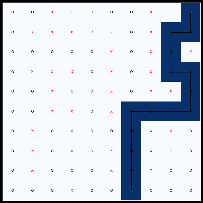
Analysis
Epsilon (Exploration Rate): Lower epsilon (0.1) leads to more consistent exploitation of learned paths. Higher values encourage more exploration but can prevent convergence to optimal paths.
Training Progress: With epsilon=0.1, gamma=0.5, and alpha=0.1, the agent:
- Early episodes: Random exploration
- 50-100 episodes: Begins finding efficient paths
- After 1000 episodes: Consistently finds goal in ~14-16 steps
Hyperparameter Effects:
- Lower epsilon values (0.1-0.2) produced better final paths
- Higher epsilon values (0.5) resulted in longer, erratic paths due to excessive exploration
- Discount factor (gamma) had less impact on this simple grid
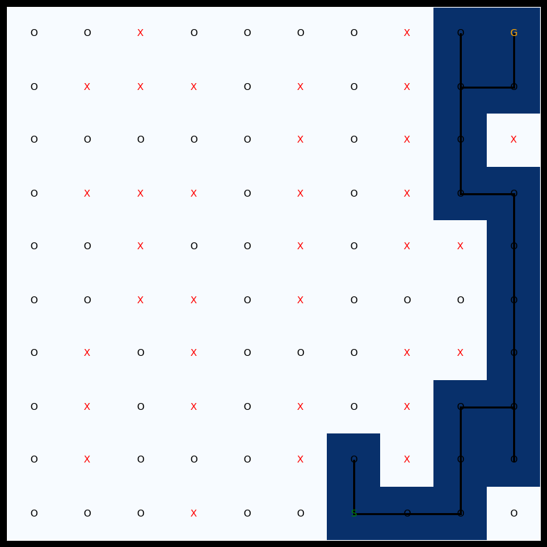
Example of suboptimal path with high exploration (epsilon=0.5, gamma=1.0): 39 steps, reward=-55
Part 2: Naive Bayes Classifier
Binary Feature Vectors
Comments are represented as binary vectors where each dimension corresponds to a word in the vocabulary (1 = present, 0 = absent).
def build_binary_vectors(file_path, vocab_size):
    vectors = {}
    with open(file_path, 'r') as file:
        for line in file:
            comment_id, word_id = map(int, line.strip().split())
            if word_id > vocab_size:
                continue
            if comment_id not in vectors:
                vectors[comment_id] = np.zeros(vocab_size, dtype=np.int8)
            vectors[comment_id][word_id - 1] = 1
    return vectors

def read_labels(file_path, comment_ids):
    labels = []
    temp_labels = {}
    with open(file_path, 'r') as file:
        for idx, line in enumerate(file):
            comment_id = idx + 1
            if comment_id in comment_ids:
                temp_labels[comment_id] = int(line.strip())
    for cid in sorted(comment_ids):
        if cid in temp_labels:
            labels.append(temp_labels[cid])
    return labels

vocab_size = 6968
train_vectors = build_binary_vectors('trainData.txt', vocab_size)
train_labels = read_labels('trainLabel.txt', train_vectors.keys())
test_vectors = build_binary_vectors('testData.txt', vocab_size)
test_labels = read_labels('testLabel.txt', test_vectors.keys())

train_X = np.array([train_vectors[cid] for cid in sorted(train_vectors.keys())])
test_X = np.array([test_vectors[cid] for cid in sorted(test_vectors.keys())])
train_y = np.array(train_labels)
test_y = np.array(test_labels)
Bernoulli Naive Bayes Implementation
def train_naive_bayes(X, y, alpha=1):
    num_samples, num_features = X.shape
    classes = np.unique(y)

    log_priors = {}
    log_prob_present = {}
    log_prob_absent = {}

    for c in classes:
        X_c = X[y == c]
        n_c = X_c.shape[0]

        # Class prior with smoothing
        log_priors[c] = np.log((n_c + alpha) / (num_samples + len(classes) * alpha))

        # P(word|class) with Laplace smoothing
        word_counts = np.sum(X_c, axis=0) + alpha
        total = n_c + (2 * alpha)
        prob_present = word_counts / total

        log_prob_present[c] = np.log(prob_present)
        log_prob_absent[c] = np.log(1.0 - prob_present)

    return log_priors, log_prob_present, log_prob_absent

def predict_naive_bayes(X_instance, log_priors, log_prob_present, log_prob_absent):
    posteriors = {}
    for c in log_priors.keys():
        log_post = log_priors[c]
        log_post += np.sum(log_prob_present[c][X_instance == 1])
        log_post += np.sum(log_prob_absent[c][X_instance == 0])
        posteriors[c] = log_post
    return max(posteriors, key=posteriors.get)

def predict_all(X, log_priors, log_prob_present, log_prob_absent):
    return np.array([predict_naive_bayes(x, log_priors, log_prob_present, log_prob_absent)
                     for x in X])

# Train and evaluate
log_priors, log_prob_present, log_prob_absent = train_naive_bayes(train_X, train_y)
train_pred = predict_all(train_X, log_priors, log_prob_present, log_prob_absent)
test_pred = predict_all(test_X, log_priors, log_prob_present, log_prob_absent)

print(f'Training Accuracy: {accuracy_score(train_y, train_pred):.4f}')
print(f'Test Accuracy: {accuracy_score(test_y, test_pred):.4f}')
print(f'Training F1: {f1_score(train_y, train_pred, average="weighted"):.4f}')
print(f'Test F1: {f1_score(test_y, test_pred, average="weighted"):.4f}')
Training Accuracy: 0.9158
Test Accuracy: 0.7434
Training F1: 0.9157
Test F1: 0.7434The classifier achieved ~91.6% training accuracy and ~74.3% test accuracy. The similarity between accuracy and F1-score indicates balanced class distribution.
Part 3: Gaussian Mixture Models for Clustering
Determining Optimal Clusters
GMMs assume data is generated from a mixture of Gaussian distributions. We use BIC and AIC to determine the optimal number of clusters.
df = pd.read_csv('Clustering Data.csv', header=None, names=['x', 'y', 'z', 'w'])

n_components_range = range(1, 11)
bic_scores = []
aic_scores = []

for k in n_components_range:
    gmm = GaussianMixture(n_components=k, random_state=0, n_init=10)
    gmm.fit(df)
    bic_scores.append(gmm.bic(df))
    aic_scores.append(gmm.aic(df))

plt.figure(figsize=(10, 5))
plt.plot(n_components_range, bic_scores, label='BIC', marker='o')
plt.plot(n_components_range, aic_scores, label='AIC', marker='x')
plt.xlabel('Number of Components')
plt.ylabel('Information Criterion Score')
plt.title('BIC and AIC for GMM')
plt.legend()
plt.grid(True)
plt.show()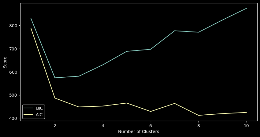
Based on the BIC/AIC curves, 2 components provides a good balance between model fit and complexity.
Clustering Results
gmm = GaussianMixture(n_components=2, random_state=0, n_init=10)
df['Cluster'] = gmm.fit_predict(df)

print(f'Number of Clusters: {df["Cluster"].nunique()}')
print('\nPoints per Cluster:')
for i, count in df['Cluster'].value_counts().sort_index().items():
    print(f'  Cluster {i}: {count}')

silhouette = silhouette_score(df[['x', 'y', 'z', 'w']], df['Cluster'])
print(f'\nSilhouette Score: {silhouette:.4f}')
Number of Clusters: 2
Points per Cluster:
Cluster 0: 100
Cluster 1: 50
Silhouette Score: 0.6986The silhouette score of ~0.70 indicates well-separated clusters. Cluster 0 contains 100 points while Cluster 1 contains 50 points.
3D Visualization
fig = plt.figure(figsize=(10, 8))
ax = fig.add_subplot(111, projection='3d')

scatter = ax.scatter(
    df['x'], df['y'], df['z'],
    c=df['Cluster'],
    cmap='viridis',
    s=df['w'] * 20,  # Size scaled by w dimension
    alpha=0.7,
    edgecolor='k',
    linewidth=0.5
)

ax.set_xlabel('X dimension')
ax.set_ylabel('Y dimension')
ax.set_zlabel('Z dimension')
ax.set_title('GMM Clustering (w dimension scales point size)')

legend_elements = [plt.Line2D([0], [0], marker='o', color='w',
                              label=f'Cluster {i}',
                              markerfacecolor=plt.cm.viridis(i / max(1, df['Cluster'].nunique()-1)),
                              markersize=8)
                   for i in sorted(df['Cluster'].unique())]
ax.legend(handles=legend_elements)

plt.show()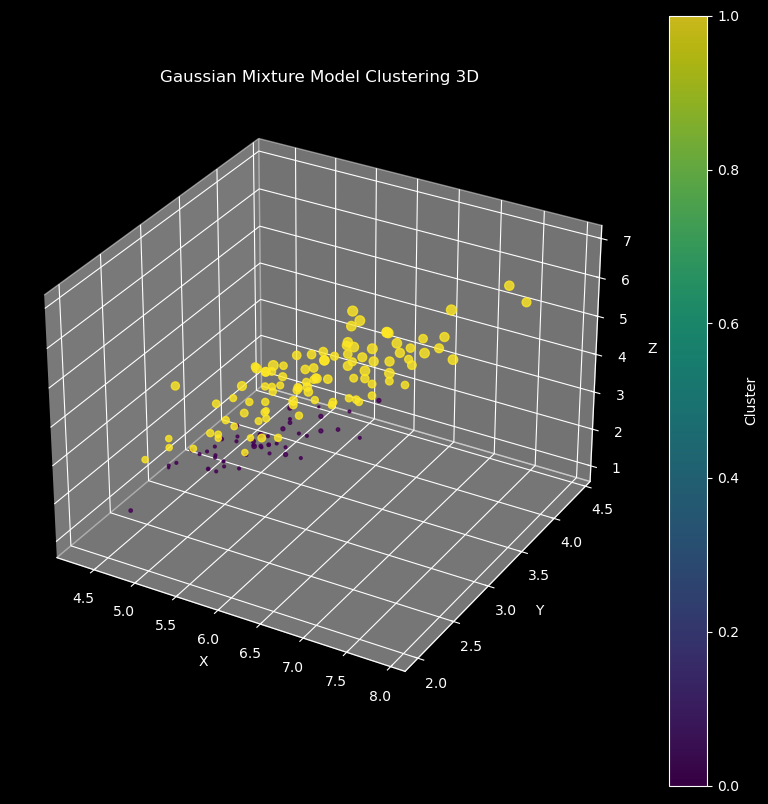
The visualization shows clear spatial separation between the two clusters in 3D space, with the fourth dimension (w) represented by point size.