Exploring Classical ML Models With PyTorch Internals
This article explores implementations of foundational machine learning models using PyTorch for core operations: K-Nearest Neighbors, Ridge Regression, and Logistic Regression.
Setup
import torch
import torch.nn as nn
import pandas as pd
import numpy as np
import matplotlib.pyplot as plt
from sklearn.model_selection import KFold
from sklearn.preprocessing import MinMaxScaler
from sklearn.metrics import accuracy_score, mean_squared_error, r2_score, f1_score
Z-Score Normalization
class ZScoreNormalizer:
    def __init__(self):
        self.mean = None
        self.std = None

    def fit(self, data):
        self.mean = torch.mean(data, dim=0)
        self.std = torch.std(data, dim=0)

    def transform(self, data):
        if self.mean is None or self.std is None:
            raise ValueError("Not fitted yet. Call fit() before transform()")

        std_safe = torch.where(self.std == 0, torch.tensor(1.0, device=self.std.device), self.std)
        return (data - self.mean) / std_safe

    def fit_transform(self, data):
        self.fit(data)
        return self.transform(data)
K-Nearest Neighbors
class KNNClassifier:
    def __init__(self):
        self.X_train = None
        self.y_train = None

    def fit(self, X_train, y_train):
        if not isinstance(X_train, torch.Tensor):
            self.X_train = torch.tensor(X_train, dtype=torch.float32)
        else:
            self.X_train = X_train.float()

        if not isinstance(y_train, torch.Tensor):
            self.y_train = torch.tensor(y_train, dtype=torch.float32)
        else:
            self.y_train = y_train.float()

    def predict(self, X_test, k):
        y_pred = []
        if not isinstance(X_test, torch.Tensor):
            X_test_tensor = torch.tensor(X_test, dtype=torch.float32)
        else:
            X_test_tensor = X_test.float()

        for x in X_test_tensor:
            distances = torch.norm(self.X_train - x, dim=1)
            indices = torch.argsort(distances)[:k]
            neighbors = self.y_train[indices]
            prediction = torch.sign(torch.sum(neighbors))
            y_pred.append(prediction.item())
        return y_pred

def knn_k_fold_cv(X, y, k_values, n_folds=10):
    train_acc, test_acc, train_err, test_err = [], [], [], []
    kf = KFold(n_splits=n_folds, shuffle=True, random_state=42)

    for k in k_values:
        fold_train_acc, fold_test_acc = [], []

        for train_idx, test_idx in kf.split(X):
            X_train, X_test = X[train_idx], X[test_idx]
            y_train, y_test = y[train_idx], y[test_idx]

            knn = KNNClassifier()
            knn.fit(X_train, y_train)

            train_pred = knn.predict(X_train, k)
            test_pred = knn.predict(X_test, k)

            fold_train_acc.append(accuracy_score(y_train, train_pred))
            fold_test_acc.append(accuracy_score(y_test, test_pred))

        train_acc.append(np.mean(fold_train_acc))
        test_acc.append(np.mean(fold_test_acc))
        train_err.append(1 - train_acc[-1])
        test_err.append(1 - test_acc[-1])

    return {"train_acc": train_acc, "test_acc": test_acc,
            "train_err": train_err, "test_err": test_err}

# Load and evaluate
input_df = pd.read_csv('KNNClassifierInput.csv', header=0)
output_df = pd.read_csv('KNNClassifierOutput.csv').dropna(axis=1)
X_data = input_df[['Input 1', 'Input 2']].values
y_data = output_df.values.squeeze()

k_values = list(range(1, 31))
results = knn_k_fold_cv(X_data, y_data, k_values, n_folds=10)

best_k_idx = np.argmax(results["test_acc"])
best_k = k_values[best_k_idx]
print(f"Best K: {best_k}")
print(f"Test Accuracy: {results['test_acc'][best_k_idx] * 100:.2f}%")

plt.figure(figsize=(10, 6))
plt.plot(k_values, results['train_acc'], label='Training Accuracy')
plt.plot(k_values, results['test_acc'], label='Testing Accuracy')
plt.axvline(best_k, color='r', linestyle='--', label=f'Best K = {best_k}')
plt.title('KNN Accuracy vs. K Value')
plt.xlabel('K (Number of Neighbors)')
plt.ylabel('Accuracy')
plt.legend()
plt.grid(True)
plt.show()
Best K: 11
Test Accuracy: 98.00%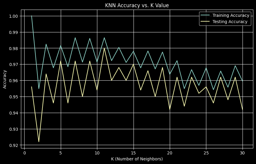
The optimal K value of 11 balances bias and variance, achieving 98% test accuracy.
Ridge Regression
class RidgeRegression(nn.Module):
    def __init__(self, input_dim):
        super(RidgeRegression, self).__init__()
        self.linear = nn.Linear(input_dim, 1)

    def forward(self, x):
        return self.linear(x)

def ridge_k_fold_cv(X, y, model_class, criterion, optimizer_class,
                    num_epochs=100, lambda_val=0.0, n_folds=5, lr=0.01):
    train_losses, test_losses, r2_scores, mse_scores = [], [], [], []
    kf = KFold(n_splits=n_folds, shuffle=True, random_state=42)

    for train_idx, test_idx in kf.split(X):
        X_train, X_test = X[train_idx], X[test_idx]
        y_train, y_test = y[train_idx], y[test_idx]

        model = model_class(X.shape[1])
        optimizer = optimizer_class(model.parameters(), lr=lr)

        if not isinstance(X_train, torch.Tensor): X_train = torch.tensor(X_train, dtype=torch.float32)
        if not isinstance(y_train, torch.Tensor): y_train = torch.tensor(y_train, dtype=torch.float32).view(-1,1)
        if not isinstance(X_test, torch.Tensor): X_test = torch.tensor(X_test, dtype=torch.float32)
        if not isinstance(y_test, torch.Tensor): y_test = torch.tensor(y_test, dtype=torch.float32).view(-1,1)

        model.train()
        for epoch in range(num_epochs):
            optimizer.zero_grad()
            outputs = model(X_train)
            loss = criterion(outputs, y_train)

            l2_reg = 0.0
            for param in model.parameters():
                if param.requires_grad and param.dim() > 1:
                    l2_reg += torch.sum(param ** 2)
            loss += lambda_val * l2_reg

            loss.backward()
            nn.utils.clip_grad_norm_(model.parameters(), max_norm=1.0)
            optimizer.step()

        model.eval()
        with torch.no_grad():
            train_out = model(X_train)
            test_out = model(X_test)
            train_losses.append(criterion(train_out, y_train).item())
            test_losses.append(criterion(test_out, y_test).item())

            y_test_np = y_test.cpu().numpy()
            test_out_np = test_out.cpu().numpy()
            r2_scores.append(r2_score(y_test_np, test_out_np))
            mse_scores.append(mean_squared_error(y_test_np, test_out_np))

    return {
        'avg_train_loss': np.mean(train_losses),
        'avg_test_loss': np.mean(test_losses),
        'avg_r2_score': np.mean(r2_scores),
        'avg_mse_score': np.mean(mse_scores)
    }

# Load and normalize data
input_df = pd.read_csv('LinearRegression.csv')
target_df = pd.read_csv('LinearRegressionTarget.csv')

X = torch.tensor(input_df.values, dtype=torch.float32)
y = torch.tensor(target_df.values, dtype=torch.float32)

normalizer_X = ZScoreNormalizer()
X_norm = normalizer_X.fit_transform(X)
normalizer_y = ZScoreNormalizer()
y_norm = normalizer_y.fit_transform(y)

# Scale lambda values
raw_lambdas = np.array(list(range(0, 251))).reshape(-1, 1)
scaler = MinMaxScaler(feature_range=(0, 1))
scaled_lambdas = scaler.fit_transform(raw_lambdas).squeeze()

results = []
for lambda_val in scaled_lambdas:
    cv_result = ridge_k_fold_cv(
        X_norm, y_norm,
        model_class=RidgeRegression,
        criterion=nn.MSELoss(),
        optimizer_class=torch.optim.SGD,
        num_epochs=100,
        lambda_val=lambda_val,
        n_folds=5,
        lr=0.01
    )
    results.append((lambda_val, cv_result))

best_lambda, best_stats = max(results, key=lambda x: x[1]['avg_r2_score'])

print(f"\nBest scaled lambda: {best_lambda:.4f}")
print(f"Best R² Score: {best_stats['avg_r2_score']:.4f}")
print(f"Best MSE: {best_stats['avg_mse_score']:.4f}")

# Plot results
r2_scores = [r[1]['avg_r2_score'] for r in results]
lambdas = [r[0] for r in results]

plt.figure(figsize=(10, 6))
plt.plot(lambdas, r2_scores)
plt.xscale('log')
plt.title('R² Score vs. Scaled Lambda (Ridge Regression)')
plt.xlabel('log(Scaled Lambda)')
plt.ylabel('Average R² Score')
plt.grid(True)
plt.show()
Best scaled lambda: 0.0360
Best R² Score: 0.9842
Best MSE: 0.0147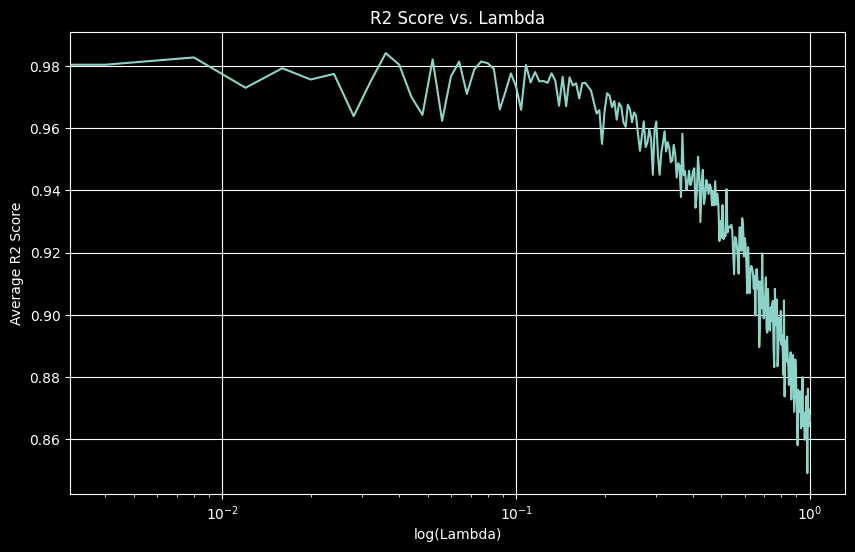
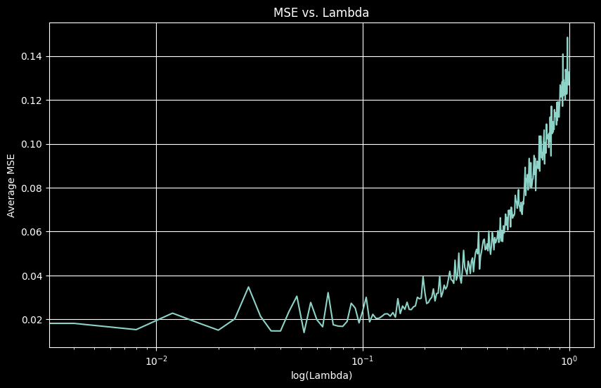
The optimal scaled λ of 0.036 (unscaled: ~9) achieved R² of 0.984, indicating minimal regularization was needed for this dataset.
Logistic Regression
class LogisticRegressionModel(nn.Module):
    def __init__(self, input_size):
        super(LogisticRegressionModel, self).__init__()
        self.linear = nn.Linear(input_size, 1)
        self.sigmoid = nn.Sigmoid()

    def forward(self, x):
        return self.sigmoid(self.linear(x))

def train_logistic_regression(X_train, y_train, num_epochs=100, lr=0.01):
    model = LogisticRegressionModel(X_train.shape[1])
    optimizer = torch.optim.SGD(model.parameters(), lr=lr)
    criterion = nn.BCELoss()

    y_train = y_train.clone().detach().float().view(-1, 1)
    train_data = torch.utils.data.TensorDataset(X_train.clone().detach().float(), y_train)
    train_loader = torch.utils.data.DataLoader(train_data, batch_size=32, shuffle=True)

    model.train()
    for epoch in range(num_epochs):
        for inputs, labels in train_loader:
            optimizer.zero_grad()
            outputs = model(inputs)
            loss = criterion(outputs, labels)
            loss.backward()
            optimizer.step()
    return model

def eval_logistic_regression(model, X_test, y_test):
    model.eval()
    y_test = y_test.clone().detach().float().view(-1, 1)
    test_data = torch.utils.data.TensorDataset(X_test.clone().detach().float(), y_test)
    test_loader = torch.utils.data.DataLoader(test_data, batch_size=32, shuffle=False)

    all_preds, all_labels = [], []
    with torch.no_grad():
        for inputs, labels in test_loader:
            outputs = model(inputs)
            preds = (outputs >= 0.5).float()
            all_preds.extend(preds.cpu().numpy().flatten())
            all_labels.extend(labels.cpu().numpy().flatten())

    acc = accuracy_score(all_labels, all_preds)
    f1 = f1_score(all_labels, all_preds, zero_division=0)
    return acc, f1, 1 - acc

def logistic_k_fold_cv(X, y, n_folds=10, num_epochs=100, lr=0.01):
    kf = KFold(n_splits=n_folds, shuffle=True, random_state=42)
    metrics = {"train_acc": [], "test_acc": [], "train_f1": [], "test_f1": [],
               "train_err": [], "test_err": []}

    for train_idx, test_idx in kf.split(X):
        X_train, X_test = X[train_idx], X[test_idx]
        y_train, y_test = y[train_idx], y[test_idx]

        model = train_logistic_regression(X_train, y_train, num_epochs, lr)

        acc_train, f1_train, err_train = eval_logistic_regression(model, X_train, y_train)
        acc_test, f1_test, err_test = eval_logistic_regression(model, X_test, y_test)

        metrics["train_acc"].append(acc_train)
        metrics["test_acc"].append(acc_test)
        metrics["train_f1"].append(f1_train)
        metrics["test_f1"].append(f1_test)
        metrics["train_err"].append(err_train)
        metrics["test_err"].append(err_test)

    return metrics

# Load and preprocess data
df = pd.read_csv("LogisticRegression.csv", names=["Input 1", "Input 2", "Input 3",
                 "Input 4", "Input 5", "Input 6", "Input 7", "Input 8", "Label"])
X_df = df.iloc[:, :-1].copy()

mode_input1 = X_df['Input 1'].mode()[0]
X_df.loc[:, 'Input 1'] = X_df['Input 1'].replace('Other', mode_input1).astype('int64')

X = torch.from_numpy(X_df.values).float()
y = torch.from_numpy(df.iloc[:, -1:].values.squeeze()).float()

normalizer = ZScoreNormalizer()
X_norm = normalizer.fit_transform(X)

results = logistic_k_fold_cv(X_norm, y, n_folds=10, lr=0.01)

print("\nLogistic Regression (10-fold CV - Mean ± Std):")
for metric, scores in results.items():
    mean, std = np.mean(scores), np.std(scores)
    print(f"{metric.replace('_', ' ').capitalize()}: {mean:.4f} (± {std:.4f})")
Logistic Regression (10-fold CV - Mean ± Std):
Train acc: 0.9602 (± 0.0003)
Test acc: 0.9600 (± 0.0018)
Train f1: 0.7274 (± 0.0015)
Test f1: 0.7260 (± 0.0130)
Train err: 0.0398 (± 0.0003)
Test err: 0.0400 (± 0.0018)Class Imbalance: This dataset is 91.5% class 0, 8.5% class 1. F1-score (~0.73) is more informative than accuracy (~96%) for evaluating minority class performance. A model predicting all 0’s would achieve 91.5% accuracy but be useless.
KNN vs Logistic Regression
Comparing both algorithms on the small KNN dataset (500 entries, 2 features).
# KNN on small dataset
input_df = pd.read_csv('KNNClassifierInput.csv', header=0)
output_df = pd.read_csv('KNNClassifierOutput.csv').dropna(axis=1)
X = input_df[['Input 1', 'Input 2']].values
y = output_df.values.squeeze()
k_values = list(range(1, 31))
knn_results = knn_k_fold_cv(X, y, k_values, n_folds=10)
best_k_idx = np.argmax(knn_results["test_acc"])
best_k = k_values[best_k_idx]
print(f"KNN - Best K: {best_k}")
print(f"KNN - Test Accuracy: {knn_results['test_acc'][best_k_idx] * 100:.2f}%")
# Logistic Regression on same dataset
y_mapped = np.where(y == -1, 0, 1)
X_tensor = torch.tensor(X, dtype=torch.float32)
y_tensor = torch.tensor(y_mapped, dtype=torch.float32)
normalizer = ZScoreNormalizer()
X_norm = normalizer.fit_transform(X_tensor)
lr_results = logistic_k_fold_cv(X_norm, y_tensor, n_folds=10, lr=0.01)
print(f"\nLogistic Regression - Mean Test Accuracy: {np.mean(lr_results['test_acc']):.4f}")
print(f"Logistic Regression - Mean Test F1: {np.mean(lr_results['test_f1']):.4f}")
# Plot comparisons
plt.figure(figsize=(10, 6))
plt.plot(k_values, knn_results["train_acc"], label='KNN Training')
plt.plot(k_values, knn_results["test_acc"], label='KNN Testing')
plt.axvline(best_k, color='r', linestyle='--', label=f'Best K = {best_k}')
plt.title('KNN Accuracy vs. K Value')
plt.xlabel('K Value')
plt.ylabel('Accuracy')
plt.legend()
plt.grid(True)
plt.show()
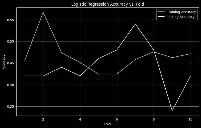
plt.figure(figsize=(10, 6))
plt.plot(range(1, 11), lr_results["train_acc"], label='Training (per fold)')
plt.plot(range(1, 11), lr_results["test_acc"], label='Testing (per fold)')
plt.title('Logistic Regression Accuracy vs. Fold')
plt.xlabel('Fold')
plt.ylabel('Accuracy')
plt.legend()
plt.grid(True)
plt.show()KNN - Best K: 13
KNN - Test Accuracy: 97.80%
Logistic Regression - Mean Test Accuracy: 0.4420
Logistic Regression - Mean Test F1: 0.1918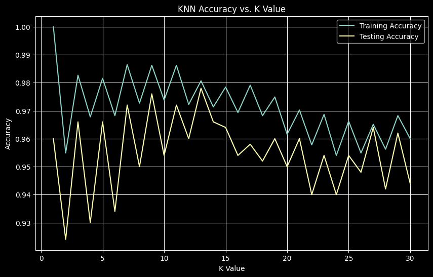
Conclusion
KNN significantly outperformed logistic regression on this small dataset (~98% vs ~44% accuracy). KNN, as an instance-based learner, effectively utilizes local information from 500 samples. Logistic regression, especially with SGD, typically requires more data to reliably converge its parameters. With limited data, performance is poor and highly variable.
Key Takeaways
- Data Normalization: Essential for distance-based (KNN) and gradient-optimized (regression) models
- Cross-Validation: Critical for hyperparameter selection and robust performance estimates
- Metric Selection: F1-score preferred over accuracy for imbalanced datasets
- Model Suitability: No free lunch - different models suit different data characteristics
- Implementation Details: Proper data type handling, model re-initialization in CV folds, and gradient clipping are important for successful training