Building Multilayer Perceptrons And Validating Them Using CIFAR-10
This article explores Feed-Forward Neural Networks (FFNNs), Deep Neural Networks (DNNs), and Multi-Layer Perceptrons (MLPs) for classifying images from the CIFAR-10 dataset, focusing on the impact of various hyperparameters and architectural choices.
Imports and Initializations
Standard libraries for deep learning, data manipulation, and plotting are imported. GPU acceleration is enabled if available.
import time
import torch
import torch.nn as nn
import torchvision as tv
import torchvision.transforms as transforms
import pandas as pd
import numpy as np
import matplotlib.pyplot as plt
from sklearn.model_selection import KFold, ParameterGrid
from sklearn.metrics import f1_score

device = torch.device("cuda" if torch.cuda.is_available() else "cpu")
classes = ('plane', 'car', 'bird', 'cat', 'deer', 'dog', 'frog', 'horse', 'ship', 'truck')
CIFAR-10 Data Loading
def load_CIFAR10(batch_size: int, raw=False):
    transform = transforms.Compose([
        transforms.ToTensor(),
        transforms.Normalize(mean=[0.5, 0.5, 0.5], std=[0.5, 0.5, 0.5])
    ])

    train_set = tv.datasets.CIFAR10(root='./data', train=True, download=True, transform=transform)
    test_set = tv.datasets.CIFAR10(root='./data', train=False, download=True, transform=transform)

    if raw:
        return train_set, test_set

    gpu_memory = torch.cuda.is_available()
    train_loader = torch.utils.data.DataLoader(
        train_set, batch_size=batch_size, shuffle=True,
        num_workers=2, pin_memory=gpu_memory
    )
    test_loader = torch.utils.data.DataLoader(
        test_set, batch_size=batch_size, shuffle=False,
        num_workers=2, pin_memory=gpu_memory
    )

    return train_loader, test_loader
Part 1: Feed-Forward Neural Network (FFNN)
FFNN Architecture
class FeedForwardNN(nn.Module):
    def __init__(self, input_size, hidden_size, num_hidden_layers, num_classes, randomize_weights=False):
        super(FeedForwardNN, self).__init__()
        self.flatten = nn.Flatten()

        layers = []
        current_size = input_size
        for _ in range(num_hidden_layers):
            layer = nn.Linear(current_size, hidden_size)
            if randomize_weights:
                nn.init.kaiming_uniform_(layer.weight, nonlinearity='sigmoid')
            else:
                nn.init.zeros_(layer.weight)
            nn.init.zeros_(layer.bias)

            layers.append(layer)
            layers.append(nn.Sigmoid())
            current_size = hidden_size

        self.hidden_layers = nn.Sequential(*layers)
        self.fc_out = nn.Linear(current_size, num_classes)

        if randomize_weights:
            nn.init.kaiming_uniform_(self.fc_out.weight, nonlinearity='sigmoid')
        else:
            nn.init.zeros_(self.fc_out.weight)
        nn.init.zeros_(self.fc_out.bias)

    def forward(self, x):
        x = self.flatten(x)
        x = self.hidden_layers(x)
        out = self.fc_out(x)
        return nn.functional.softmax(out, dim=1)
Training and Testing Functions
def test_ffnn_model(test_loader, input_size, model):
    model.eval()
    with torch.no_grad():
        total_correct = 0
        total_samples = 0
        for images, labels in test_loader:
            images = images.to(device)
            labels = labels.to(device)
            outputs = model(images)
            _, predicted = torch.max(outputs.data, 1)
            total_samples += labels.size(0)
            total_correct += (predicted == labels).sum().item()

        accuracy = 100 * total_correct / total_samples
        return 100 - accuracy

def train_and_test_ffnn(input_size, train_loader, test_loader, hidden_size,
                        num_classes, num_hidden_layers, num_epochs,
                        learning_rate, randomize_weights=False):
    model = FeedForwardNN(input_size, hidden_size, num_hidden_layers,
                          num_classes, randomize_weights=randomize_weights)
    model.to(device)
    criterion = nn.CrossEntropyLoss()
    optimizer = torch.optim.SGD(model.parameters(), lr=learning_rate)

    train_error_rates, test_error_rates = [], []

    for epoch in range(num_epochs):
        model.train()
        total_correct_train = 0
        total_samples_train = 0

        for images, labels in train_loader:
            images = images.to(device)
            labels = labels.to(device)

            optimizer.zero_grad()
            outputs = model(images)
            loss = criterion(outputs, labels)
            loss.backward()
            optimizer.step()

            _, predicted = torch.max(outputs.data, 1)
            total_samples_train += labels.size(0)
            total_correct_train += (predicted == labels).sum().item()

        train_accuracy = 100 * total_correct_train / total_samples_train
        train_error_rates.append(100 - train_accuracy)
        test_error_rates.append(test_ffnn_model(test_loader, input_size, model))

    return train_error_rates, test_error_rates
Baseline Configuration
input_size_ffnn = 3 * 32 * 32
batch_size_ffnn = 200
hidden_size_ffnn = 300
num_classes_ffnn = 10
num_hidden_layers_ffnn = 1
num_epochs_ffnn_baseline = 10
learning_rate_ffnn = 0.01
randomize_weights_ffnn = True

train_loader_ffnn, test_loader_ffnn = load_CIFAR10(batch_size=batch_size_ffnn)

train_err_baseline, test_err_baseline = train_and_test_ffnn(
    input_size_ffnn, train_loader_ffnn, test_loader_ffnn,
    hidden_size_ffnn, num_classes_ffnn, num_hidden_layers_ffnn,
    num_epochs_ffnn_baseline, learning_rate_ffnn, randomize_weights_ffnn
)

plt.figure(figsize=(10, 6))
plt.plot(train_err_baseline, label='Training Error Rate')
plt.plot(test_err_baseline, label='Test Error Rate')
plt.xlabel('Epochs')
plt.ylabel('Error Rate (%)')
plt.title('FFNN Baseline Performance (Batch Size 200, 10 Epochs)')
plt.legend()
plt.grid(True)
plt.show()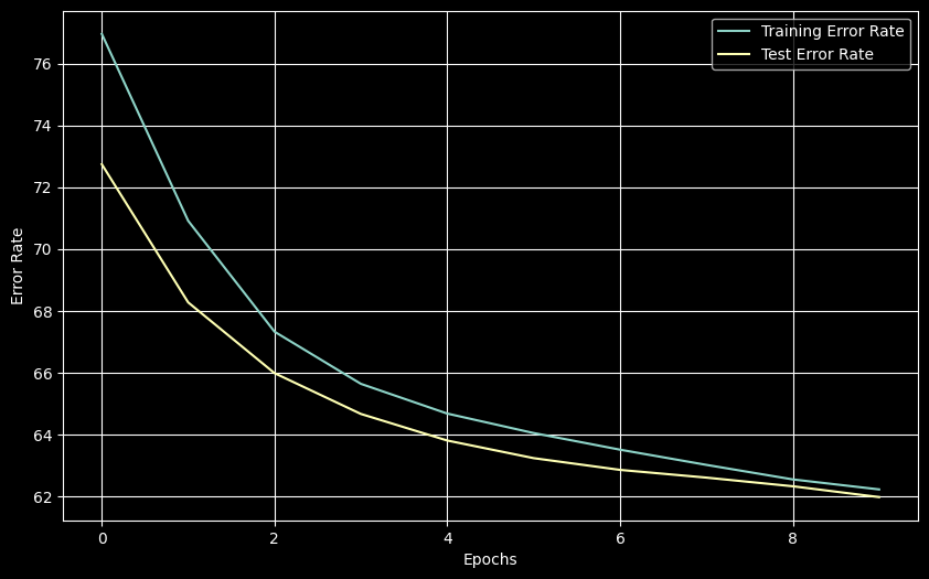
The baseline shows typical learning behavior with training and test errors decreasing and converging over 10 epochs.
Impact of Training Epochs
epochs_to_test = [10, 20, 30, 40, 50]
final_train_errors, final_test_errors = [], []

for epochs_val in epochs_to_test:
    train_results, test_results = train_and_test_ffnn(
        input_size_ffnn, train_loader_ffnn, test_loader_ffnn,
        hidden_size_ffnn, num_classes_ffnn, num_hidden_layers_ffnn,
        epochs_val, learning_rate_ffnn, randomize_weights_ffnn
    )
    final_train_errors.append(train_results[-1])
    final_test_errors.append(test_results[-1])

plt.figure(figsize=(10, 6))
plt.plot(epochs_to_test, final_train_errors, label='Training Error', marker='o')
plt.plot(epochs_to_test, final_test_errors, label='Test Error', marker='x')
plt.xlabel('Number of Epochs')
plt.ylabel('Final Error Rate (%)')
plt.title('FFNN Error Rate vs. Number of Epochs')
plt.legend()
plt.grid(True)
plt.show()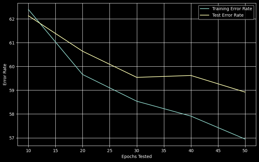
Increasing epochs reduces both training and test error, with the lowest test error (58.92%) at 50 epochs.
Impact of Hidden Layer Size
hidden_sizes_to_test = [2, 4, 15, 40, 250, 300]
final_train_errors, final_test_errors = [], []

for hs_val in hidden_sizes_to_test:
    train_results, test_results = train_and_test_ffnn(
        input_size_ffnn, train_loader_ffnn, test_loader_ffnn,
        hs_val, num_classes_ffnn, num_hidden_layers_ffnn,
        50, learning_rate_ffnn, randomize_weights_ffnn
    )
    final_train_errors.append(train_results[-1])
    final_test_errors.append(test_results[-1])

plt.figure(figsize=(10, 6))
plt.plot(hidden_sizes_to_test, final_train_errors, label='Training Error', marker='o')
plt.plot(hidden_sizes_to_test, final_test_errors, label='Test Error', marker='x')
plt.xlabel('Number of Hidden Nodes (1 Layer)')
plt.ylabel('Final Error Rate (%)')
plt.title('FFNN Error Rate vs. Number of Hidden Nodes')
plt.legend()
plt.grid(True)
plt.show()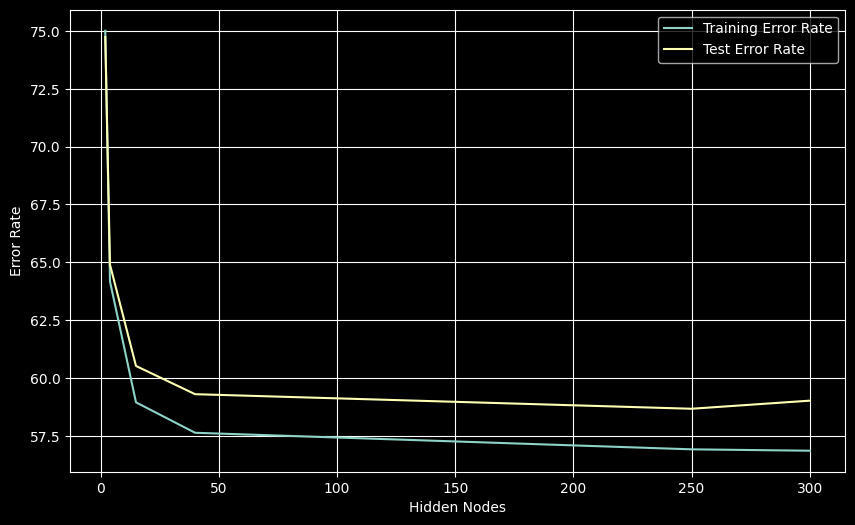
Error rates decrease with more hidden nodes. Best test error (58.67%) achieved with 250 nodes.
Weight Initialization Comparison
# Random vs. zero weight initialization
train_err_random, test_err_random = train_and_test_ffnn(
    input_size_ffnn, train_loader_ffnn, test_loader_ffnn,
    250, num_classes_ffnn, num_hidden_layers_ffnn,
    50, learning_rate_ffnn, randomize_weights=True
)

train_err_zero, test_err_zero = train_and_test_ffnn(
    input_size_ffnn, train_loader_ffnn, test_loader_ffnn,
    250, num_classes_ffnn, num_hidden_layers_ffnn,
    50, learning_rate_ffnn, randomize_weights=False
)

plt.figure(figsize=(12, 7))
plt.plot(train_err_random, label='Random Weights - Training')
plt.plot(test_err_random, label='Random Weights - Test')
plt.plot(train_err_zero, label='Zero Weights - Training', linestyle='--')
plt.plot(test_err_zero, label='Zero Weights - Test', linestyle='--')
plt.xlabel('Epoch')
plt.ylabel('Error Rate (%)')
plt.title('FFNN Error Rate: Random vs. Zero Weight Initialization')
plt.legend()
plt.grid(True)
plt.show()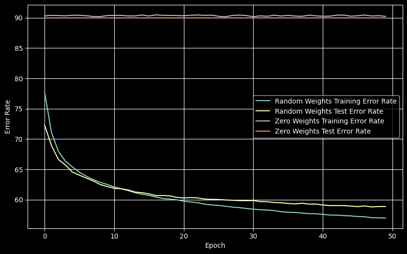
Zero initialization causes a symmetry problem where all neurons learn identical features, resulting in ~90% error (random guessing). Random initialization is essential for breaking symmetry.
Impact of Learning Rate
learning_rates_to_test = [0.0005, 0.05, 0.1, 0.15, 0.25, 0.5]
final_train_errors, final_test_errors = [], []

for lr_val in learning_rates_to_test:
    train_results, test_results = train_and_test_ffnn(
        input_size_ffnn, train_loader_ffnn, test_loader_ffnn,
        250, num_classes_ffnn, num_hidden_layers_ffnn,
        50, lr_val, randomize_weights=True
    )
    final_train_errors.append(train_results[-1])
    final_test_errors.append(test_results[-1])

plt.figure(figsize=(10, 6))
plt.plot(learning_rates_to_test, final_train_errors, label='Training Error', marker='o')
plt.plot(learning_rates_to_test, final_test_errors, label='Test Error', marker='x')
plt.xlabel('Learning Rate')
plt.ylabel('Final Error Rate (%)')
plt.title('FFNN Error Rate vs. Learning Rate')
plt.legend()
plt.grid(True)
plt.show()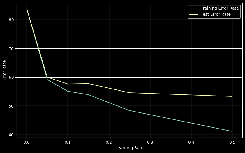
Higher learning rates (up to 0.5) improved performance, achieving best test error (53.29%) at LR=0.5. The widening gap between training and test error suggests increased overfitting at higher learning rates.
Impact of Network Depth
num_hidden_layers_to_test = [1, 3, 5, 7]
final_train_errors, final_test_errors = [], []

for nhl_val in num_hidden_layers_to_test:
    train_results, test_results = train_and_test_ffnn(
        input_size_ffnn, train_loader_ffnn, test_loader_ffnn,
        250, num_classes_ffnn, nhl_val,
        50, 0.5, randomize_weights=True
    )
    final_train_errors.append(train_results[-1])
    final_test_errors.append(test_results[-1])

plt.figure(figsize=(10, 6))
plt.plot(num_hidden_layers_to_test, final_train_errors, label='Training Error', marker='o')
plt.plot(num_hidden_layers_to_test, final_test_errors, label='Test Error', marker='x')
plt.xlabel('Number of Hidden Layers')
plt.ylabel('Final Error Rate (%)')
plt.title('FFNN Error Rate vs. Number of Hidden Layers (Sigmoid)')
plt.legend()
plt.grid(True)
plt.xticks(num_hidden_layers_to_test)
plt.show()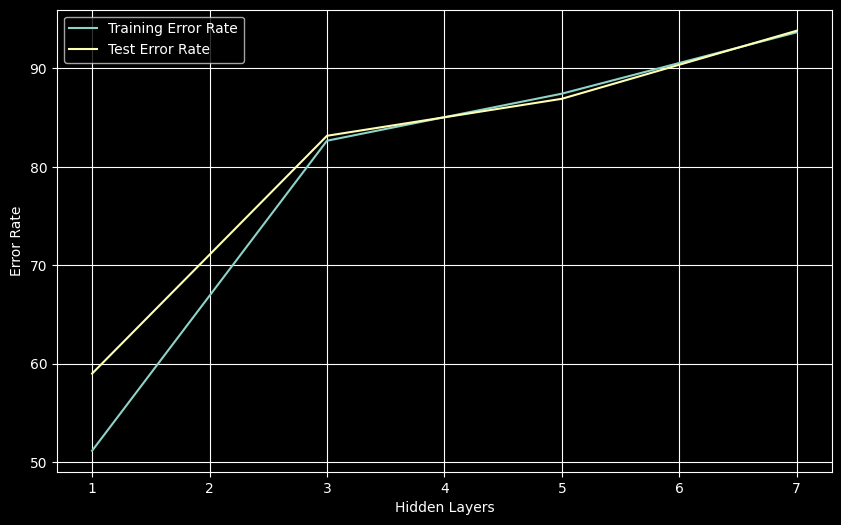
Performance degrades dramatically with more layers, reaching ~90% error (random guessing) with 5+ layers. This is the classic vanishing gradient problem with sigmoid activations - gradients become too small during backpropagation through many layers, preventing effective learning.
Part 2: Deep Neural Network with ReLU
ReLU activation addresses the vanishing gradient problem observed with sigmoid networks.
DNN Architecture
class DeepNN(nn.Module):
    def __init__(self, input_size, hidden_size, num_hidden_layers, num_classes):
        super(DeepNN, self).__init__()
        self.flatten = nn.Flatten()

        layers = []
        current_size = input_size
        for _ in range(num_hidden_layers):
            layer = nn.Linear(current_size, hidden_size)
            nn.init.kaiming_uniform_(layer.weight, nonlinearity='relu')
            nn.init.zeros_(layer.bias)
            layers.append(layer)
            layers.append(nn.ReLU())
            current_size = hidden_size

        self.hidden_layers = nn.Sequential(*layers)
        self.fc_out = nn.Linear(current_size, num_classes)
        nn.init.kaiming_uniform_(self.fc_out.weight, nonlinearity='relu')
        nn.init.zeros_(self.fc_out.bias)

    def forward(self, x):
        x = self.flatten(x)
        x = self.hidden_layers(x)
        out = self.fc_out(x)
        return nn.functional.softmax(out, dim=1)

def train_and_test_dnn(input_size, train_loader, test_loader, hidden_size,
                       num_classes, num_hidden_layers, num_epochs, learning_rate):
    model = DeepNN(input_size, hidden_size, num_hidden_layers, num_classes)
    model.to(device)
    criterion = nn.CrossEntropyLoss()
    optimizer = torch.optim.SGD(model.parameters(), lr=learning_rate)

    train_error_rates, test_error_rates = [], []

    for epoch in range(num_epochs):
        model.train()
        total_correct_train = 0
        total_samples_train = 0

        for images, labels in train_loader:
            images = images.to(device)
            labels = labels.to(device)

            optimizer.zero_grad()
            outputs = model(images)
            loss = criterion(outputs, labels)
            loss.backward()
            optimizer.step()

            _, predicted = torch.max(outputs.data, 1)
            total_samples_train += labels.size(0)
            total_correct_train += (predicted == labels).sum().item()

        train_accuracy = 100 * total_correct_train / total_samples_train
        train_error_rates.append(100 - train_accuracy)

        model.eval()
        with torch.no_grad():
            total_correct = 0
            total_samples = 0
            for images, labels in test_loader:
                images = images.to(device)
                labels = labels.to(device)
                outputs = model(images)
                _, predicted = torch.max(outputs.data, 1)
                total_samples += labels.size(0)
                total_correct += (predicted == labels).sum().item()
            test_error_rates.append(100 - 100 * total_correct / total_samples)

    return train_error_rates, test_error_rates
DNN Performance with FFNN Hyperparameters
train_loader_dnn, test_loader_dnn = load_CIFAR10(batch_size=200)
epochs_dnn_sweep = [10, 20, 30, 40, 50]
final_train_errors, final_test_errors = [], []

for epochs_val in epochs_dnn_sweep:
    train_results, test_results = train_and_test_dnn(
        3*32*32, train_loader_dnn, test_loader_dnn,
        250, 10, 1, epochs_val, 0.5
    )
    final_train_errors.append(train_results[-1])
    final_test_errors.append(test_results[-1])

plt.figure(figsize=(10, 6))
plt.plot(epochs_dnn_sweep, final_train_errors, label='Training Error', marker='o')
plt.plot(epochs_dnn_sweep, final_test_errors, label='Test Error', marker='x')
plt.xlabel('Number of Epochs')
plt.ylabel('Final Error Rate (%)')
plt.title('DNN (ReLU) Performance with FFNN Optimal Hyperparameters')
plt.legend()
plt.grid(True)
plt.show()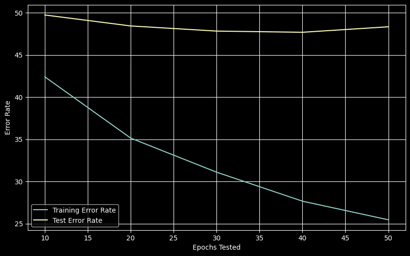
ReLU activation significantly improves performance: best test error of 47.69% at 40 epochs, compared to 53.13% for the sigmoid FFNN.
K-Fold Cross-Validation with F1-Score
def validate_test_f1(model, target_loader, criterion):
    model.eval()
    total_loss = 0.0
    all_predictions, all_labels = [], []
    with torch.no_grad():
        for images, labels in target_loader:
            images = images.to(device)
            labels = labels.to(device)
            outputs = model(images)
            loss = criterion(outputs, labels)
            total_loss += loss.item() * images.size(0)
            all_predictions.extend(outputs.argmax(dim=1).cpu().numpy())
            all_labels.extend(labels.cpu().numpy())

    avg_loss = total_loss / len(target_loader.dataset)
    f1 = f1_score(all_labels, all_predictions, average='weighted', zero_division=0)
    return f1, avg_loss

def train_f1(model, train_loader, criterion, optimizer):
    model.train()
    total_loss = 0.0
    all_predictions, all_labels = [], []
    for images, labels in train_loader:
        images = images.to(device)
        labels = labels.to(device)
        optimizer.zero_grad()
        outputs = model(images)
        loss = criterion(outputs, labels)
        loss.backward()
        optimizer.step()
        total_loss += loss.item() * images.size(0)
        all_predictions.extend(outputs.argmax(dim=1).cpu().numpy())
        all_labels.extend(labels.cpu().numpy())

    avg_loss = total_loss / len(train_loader.dataset)
    f1 = f1_score(all_labels, all_predictions, average='weighted', zero_division=0)
    return f1, avg_loss

def kfold_train_optimize(input_dim, batch_s, param_grid, num_epochs, model_class):
    kfold = KFold(n_splits=5, shuffle=True, random_state=42)
    raw_train_set, raw_test_set = load_CIFAR10(batch_size=batch_s, raw=True)

    best_params = None
    best_val_f1 = -1.0
    best_avg_losses = {'train': float('inf'), 'val': float('inf'), 'test': float('inf')}
    best_avg_f1s = {'train': 0, 'val': 0, 'test': 0}
    best_fold_f1_data = {}
    best_fold_loss_data = {}

    for params in ParameterGrid(param_grid):
        fold_f1s = {'train': [], 'val': [], 'test': []}
        fold_losses = {'train': [], 'val': [], 'test': []}

        for fold_idx, (train_indices, val_indices) in enumerate(kfold.split(raw_train_set)):
            train_subset = torch.utils.data.Subset(raw_train_set, train_indices)
            val_subset = torch.utils.data.Subset(raw_train_set, val_indices)

            train_loader = torch.utils.data.DataLoader(train_subset, batch_size=batch_s,
                                                       shuffle=True, pin_memory=torch.cuda.is_available())
            val_loader = torch.utils.data.DataLoader(val_subset, batch_size=batch_s,
                                                     shuffle=False, pin_memory=torch.cuda.is_available())
            test_loader = torch.utils.data.DataLoader(raw_test_set, batch_size=batch_s,
                                                      shuffle=False, pin_memory=torch.cuda.is_available())

            model = model_class(input_dim, params['hidden_size'],
                              params['num_hidden_layers'], params['num_classes'])
            model.to(device)
            criterion = nn.CrossEntropyLoss()
            optimizer = torch.optim.SGD(model.parameters(), lr=params['learning_rate'])

            for epoch in range(num_epochs):
                train_f1_epoch, train_loss_epoch = train_f1(model, train_loader, criterion, optimizer)

            val_f1, val_loss = validate_test_f1(model, val_loader, criterion)
            test_f1, test_loss = validate_test_f1(model, test_loader, criterion)

            fold_f1s['train'].append(train_f1_epoch)
            fold_f1s['val'].append(val_f1)
            fold_f1s['test'].append(test_f1)
            fold_losses['train'].append(train_loss_epoch)
            fold_losses['val'].append(val_loss)
            fold_losses['test'].append(test_loss)

        avg_val_f1 = np.mean(fold_f1s['val'])
        if avg_val_f1 > best_val_f1:
            best_val_f1 = avg_val_f1
            best_params = params.copy()
            for key in ['train', 'val', 'test']:
                best_avg_f1s[key] = np.mean(fold_f1s[key])
                best_avg_losses[key] = np.mean(fold_losses[key])
            best_fold_f1_data = fold_f1s.copy()
            best_fold_loss_data = fold_losses.copy()

    return best_avg_losses, best_avg_f1s, best_params, [best_fold_f1_data], [best_fold_loss_data]
K-Fold Results
dnn_kfold_param_grid = {
    'hidden_size': [250],
    'num_hidden_layers': [1],
    'num_classes': [10],
    'learning_rate': [0.5],
}

avg_losses, avg_f1_scores, winning_params, fold_f1_list, fold_loss_list = \
    kfold_train_optimize(3*32*32, 200, dnn_kfold_param_grid, 50, DeepNN)

fold_f1_data = fold_f1_list[0]
fold_loss_data = fold_loss_list[0]

plt.figure(figsize=(10, 6))
plt.plot(range(1, 6), fold_f1_data['train'], label='Training F1', marker='o')
plt.plot(range(1, 6), fold_f1_data['val'], label='Validation F1', marker='x')
plt.plot(range(1, 6), fold_f1_data['test'], label='Test F1', marker='s')
plt.xlabel('Fold')
plt.ylabel('F1 Score')
plt.title('DNN K-Fold CV: F1 Scores per Fold')
plt.legend()
plt.grid(True)
plt.xticks(range(1,6))
plt.show()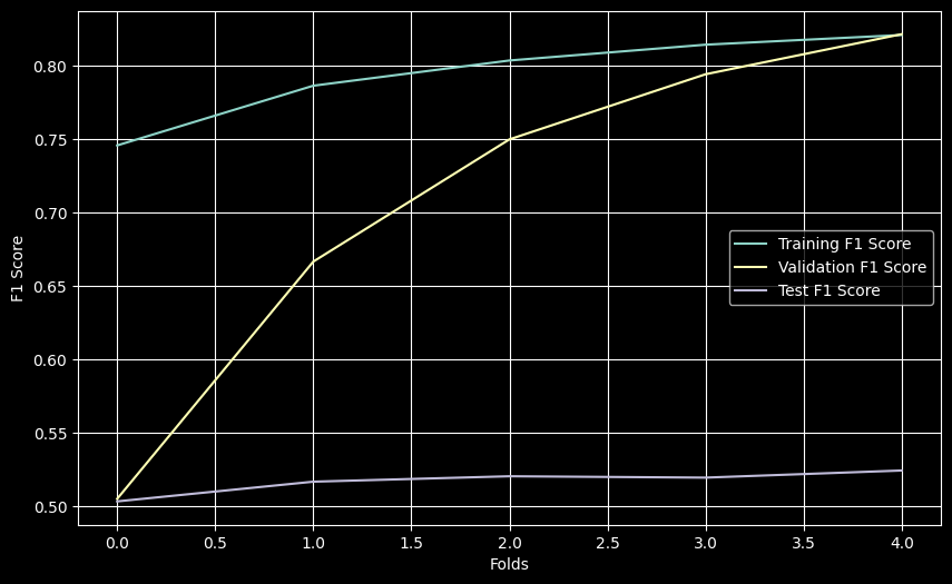
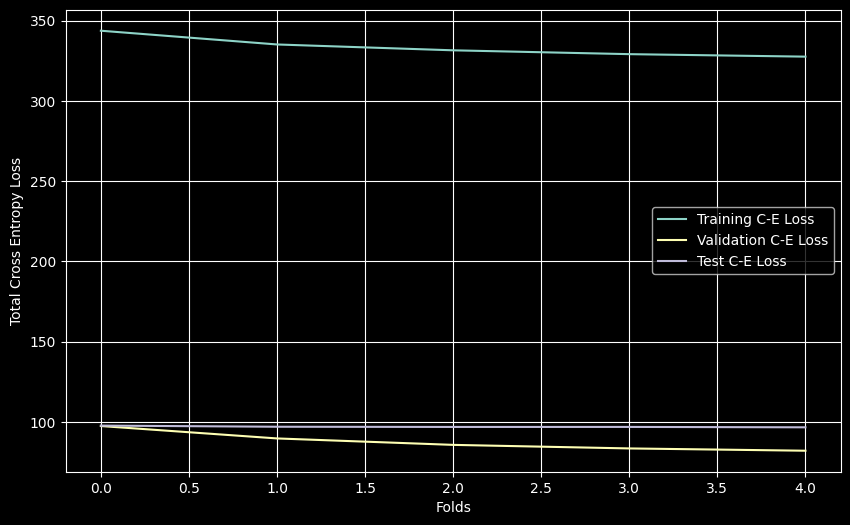
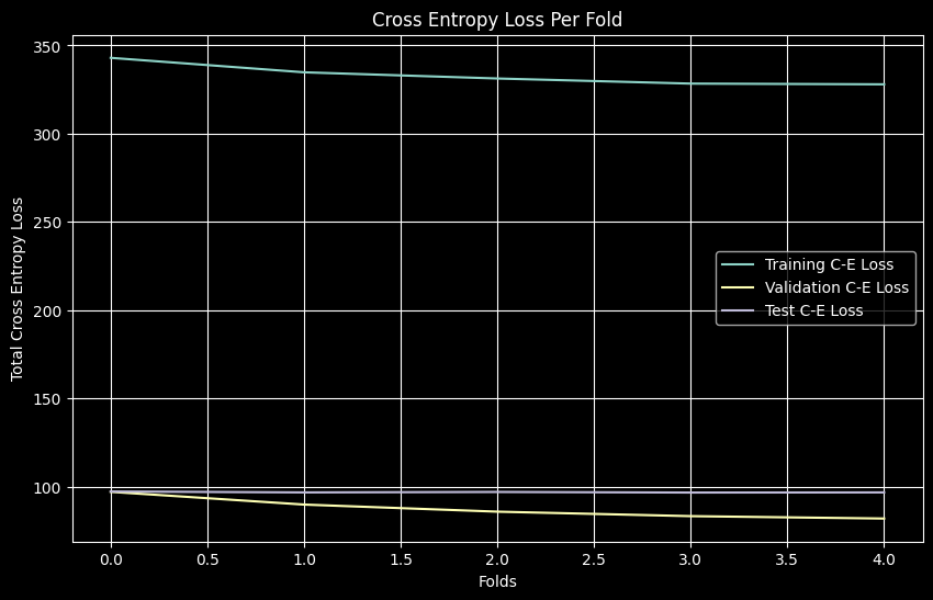
K-Fold results show strong F1 scores on training/validation (~0.82) but significantly lower test F1 (~0.52), indicating overfitting.
Part 3: Multi-Layer Perceptron
The MLP architecture is identical to the DNN (ReLU activation). Both effectively use mini-batch gradient descent.
class MLP(nn.Module):
    def __init__(self, input_size, hidden_size, num_hidden_layers, num_classes):
        super(MLP, self).__init__()
        self.flatten = nn.Flatten()
        layers = []
        current_size = input_size
        for _ in range(num_hidden_layers):
            layer = nn.Linear(current_size, hidden_size)
            nn.init.kaiming_uniform_(layer.weight, nonlinearity='relu')
            nn.init.zeros_(layer.bias)
            layers.append(layer)
            layers.append(nn.ReLU())
            current_size = hidden_size
        self.hidden_layers = nn.Sequential(*layers)
        self.fc_out = nn.Linear(current_size, num_classes)
        nn.init.kaiming_uniform_(self.fc_out.weight, nonlinearity='relu')
        nn.init.zeros_(self.fc_out.bias)

    def forward(self, x):
        x = self.flatten(x)
        x = self.hidden_layers(x)
        out = self.fc_out(x)
        return nn.functional.softmax(out, dim=1)

mlp_kfold_param_grid = {
    'hidden_size': [250],
    'num_hidden_layers': [1],
    'num_classes': [10],
    'learning_rate': [0.5],
}

avg_losses_mlp, avg_f1_scores_mlp, winning_params_mlp, \
fold_f1_list_mlp, fold_loss_list_mlp = \
    kfold_train_optimize(3*32*32, 200, mlp_kfold_param_grid, 50, MLP)

fold_f1_data_mlp = fold_f1_list_mlp[0]

plt.figure(figsize=(10, 6))
plt.plot(range(1, 6), fold_f1_data_mlp['train'], label='Training F1', marker='o')
plt.plot(range(1, 6), fold_f1_data_mlp['val'], label='Validation F1', marker='x')
plt.plot(range(1, 6), fold_f1_data_mlp['test'], label='Test F1', marker='s')
plt.xlabel('Fold')
plt.ylabel('F1 Score')
plt.title('MLP K-Fold CV: F1 Scores per Fold')
plt.legend()
plt.grid(True)
plt.xticks(range(1,6))
plt.show()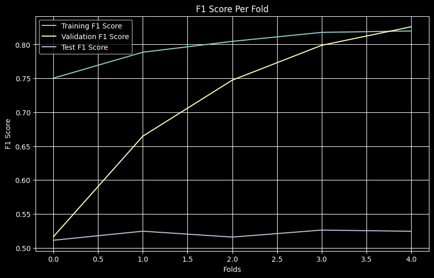
MLP results are nearly identical to DNN (Train F1 ~0.82, Val F1 ~0.83, Test F1 ~0.52), as expected given identical architectures and training.
Conclusions
Performance Comparison
DNN vs MLP K-Fold Results:
- F1 Scores (Averaged): DNN (Train ~0.82, Val ~0.82, Test ~0.52) vs MLP (Train ~0.82, Val ~0.83, Test ~0.52)
- Cross-Entropy Loss (Averaged): DNN (Train ~1.64, Val ~1.64, Test ~1.95) vs MLP (Train ~1.64, Val ~1.64, Test ~1.95)
The near-identical results confirm that architecture and activation function choice matter more than naming conventions.
Key Findings
-
ReLU vs. Sigmoid: ReLU activation dramatically improved performance. Test error dropped from ~53% (sigmoid FFNN) to ~48% (ReLU DNN) with comparable hyperparameters, demonstrating ReLU’s effectiveness in mitigating vanishing gradients.
-
Overfitting: Both ReLU-based models showed significant overfitting when using FFNN-derived hyperparameters (training/validation F1 ~82%, test F1 ~52%). This suggests that regularization techniques (dropout, weight decay) or different hyperparameters are needed for better generalization.
-
Vanishing Gradients: The sigmoid FFNN’s performance collapsed with deeper networks (>3 layers), reaching ~90% error (random guessing). This classic vanishing gradient problem occurs when gradients become too small during backpropagation through many sigmoid layers.
-
Weight Initialization: Random weight initialization is essential. Zero initialization caused complete failure (~90% error) due to symmetry problems where all neurons learn identical features.
-
Limitations for Image Classification: These fully-connected architectures are fundamentally limited for image tasks because they don’t capture spatial hierarchies or translation invariance. Convolutional Neural Networks (CNNs) would significantly outperform these approaches on CIFAR-10.
Recommendations
For improved performance on CIFAR-10:
- Use CNN architectures designed for spatial data
- Apply regularization (dropout, L2 regularization)
- Implement learning rate scheduling
- Consider data augmentation
- Perform comprehensive hyperparameter tuning with grid search or Bayesian optimization